What can one wind line determine?

Start from saved integer photons

The exercise saves integer counts in 256 velocity bins, their width, continuum-photon calibration and instrument response. This is a synthetic photon detector. IUE ABS_CAL is processed energy flux and cannot become a Poisson count record merely by renaming a column.

First calculate the wind photon spectrum, convolve it with the fixed instrument Gaussian and integrate each bin. Generate counts only afterward. This permits the instrument to distribute photons among adjacent bins. Adding noise before arbitrary smoothing would produce a different noise correlation.

The conditional example fixes beta exponent one, asymptotic speed 200 kilometres per second, aperture eight stellar radii, instrument standard deviation eight kilometres per second and continuum calibration 1600 photons per kilometre per second. Instrument width is separate from thermal wind width.

Reading: Standalone stellar-wind scientific reproduction

Write the probability of those counts

A Poisson distribution describes the count obtained when the mean arrival number is known. For mean $\lambda_i$, the probability of observing $N_i$ photons follows the expression below. Multiply the conditional probabilities across bins to obtain the likelihood of the whole saved spectrum.

Taking logarithms changes products into sums. The factorial term is constant across parameters for one fixed dataset and may be omitted from relative parameter comparisons. It remains part of the original probability distribution. Square-root-count error bars are a large-count approximation; inference here retains the Poisson expression.

infer_saved_counts receives saved counts and the means of a declared model family. Generating truths are saved separately and read afterward for coverage validation. Editing a truth annotation cannot change the inferred result.

Reading: Standalone stellar-wind scientific reproduction

Two physically different flows can have the same line

Define mass-flow multiplier $m=\dot M/\dot M_{\rm ref}$ and relative line-opacity multiplier $q$. The latter can represent relative ionization, abundance or level-population changes; it is not an absolute ion fraction. At fixed velocity and geometry, optical depth depends on their product $\theta=mq$.

Mass multiplier one with opacity multiplier one therefore gives the same photon profile as half the mass flow with twice the opacity. With the same noise realization, even the saved integer bins coincide. Density differs, but this line has not measured it separately.

The force diagnostic cannot casually be promoted to an extra observation that breaks the degeneracy. The flow is prescribed, the one-line force is insufficient and other forces are absent. Adding a dynamical constraint requires the relevant physics and evidence.

Reading: Lamers, Cerruti-Sola & Perinotto1987, the SEI line-profile method · Standalone stellar-wind scientific reproduction

Transform the proper two-parameter prior

Assign independent LogUniform priors from 0.5 to 2 to both $m$ and $q$. Equal intervals in their logarithms have equal prior probability. With $x=\ln m$, $y=\ln q$ and $a=\ln2$, both log coordinates are uniform on $[-a,a]$.

Returning to linear coordinates requires a Jacobian. The resulting joint density contains the two parameters in its denominator. Dropping that factor would select a different prior.

Now set $s=x+y=\ln\theta$. The number of allowed parameter pairs at a given sum is proportional to a diagonal segment through the log-coordinate square. Segments are longest centrally and vanish at the ends, producing a triangular log-product prior. Linear product density requires an additional division by $\theta$.

Multiply likelihood by this prior and normalize to form the posterior. A mass-flow marginal integrates over all allowed opacity multipliers. Fixing opacity to one instead asks a different conditional question.

Reading: Standalone stellar-wind scientific reproduction

Work through the saved observation

The default record contains 872258 photons. Its calibrated absorption-positive velocity equivalent width is about 14.84 kilometres per second. Counting noise alone gives an estimated standard deviation about 0.584 kilometres per second, conditional on the known continuum. Continuum and physical-model uncertainty are additional questions.

Standalone Python recomputes transfer, convolution and binning. Across the full product support, the total mean discrepancy from finer calculations is about 0.009 Poisson-noise units. Product grids with 1201 and 2401 points change interval endpoints by less than 0.6 percent of the interval width.

The product posterior has median about 0.991 and central 95 percent interval about 0.974 to 1.009. The mass-flow multiplier interval remains about 0.518 to 1.914, nearly spanning its original 0.5 to 2 range. The opacity marginal is identical because the likelihood and priors are symmetric under exchanging the two parameters.

The narrow ridge in the figure is a collection of answers with almost the same product. Its wide mass-flow range and its boundaries depend strongly on the prior. This is not a separate precise mass-loss measurement.

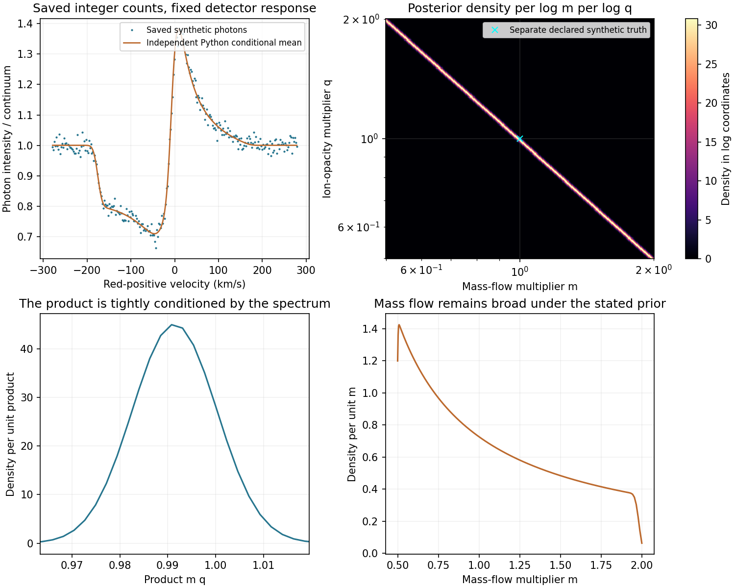
python3 conditional_count_inference.py --measurement measurement/synthetic-photon-measurement.json --out-dir rerun

Reading: Standalone stellar-wind scientific reproduction

Test prior-averaged and fixed-truth coverage separately

A central 95 percent credible interval is a posterior statement given data and prior: 2.5 percent probability lies in each excluded tail. It does not automatically promise 95 percent repeated-experiment coverage at every fixed true parameter.

The first check draws true mass and opacity independently from the stated priors, then generates 240 independent Poisson observations. Product intervals cover 232 times; mass-flow intervals cover 227 times. Binomial uncertainty accompanies those counts. This tests coverage averaged over the declared prior.

The second check fixes three parameter pairs: $(m,q)=(1,1)$, $(0.51,0.51)$ and $(1.99,0.51)$. Each has 100 independently generated records. Product coverage is 94, 95 and 95; mass-flow coverage is 100, 100 and zero. Original counts and these failures are retained.

The final pair has product about 1.015, close to the central case, but mass near its prior boundary. The spectrum constrains the product; prior volume and marginalization allocate mass along the ridge. A central interval can repeatedly exclude the fixed mass value 1.99 after trimming its boundary tails.

Zero coverage in that case is not an unlucky precise mass-loss measurement. It exposes non-identifiability and failure of a universal fixed-parameter coverage interpretation. Both the prior-averaged and fixed-truth results belong beside the posterior plot.

Reading: Standalone stellar-wind scientific reproduction

Identify the additional conditions needed for real data

Real continuum, response, ion populations, velocity law and interstellar absorption may be unknown, and lines can overlap. They change the predicted mean, its errors and parameter relationships. Reducing synthetic counting noise cannot by itself remove a product degeneracy.

IUE energy flux and its FN noise are at different calibration stages. They do not provide this exercise with independent Poisson counts and a complete physical-error vector. The next tutorial retains native orders, quality gaps and continuum sensitivity, then compares shapes under explicit isolated-line conditions. Real mass-loss work needs multiple diagnostics and a corresponding atmosphere model.

Reading: IUE NEWSIPS manual, high-dispersion MXHI format · IUE data-analysis FAQ · Brands, Backs, de Koter et al.2025, X-Shooting ULLYSES XII