Replaying the IUE ultraviolet spectra of P Cygni

Identify the three observations

P Cygni is HD193237. SWP36331 was observed on 23 May 1989 for 2999.781 seconds; LWP15586 followed on 24 May for 239.493 seconds. They cover different ultraviolet bands. Their dates are close, but they are not a simultaneous exposure of the same spectrum.

LWP04483 is a separate long-wavelength observation from 2 October 1984, exposed for 299.704 seconds. Use it to inspect change between epochs. Verify the complete bytes and SHA before reading the target, observing date, exposure and processing date from the header. A NEWSIPS processing date in 1997 is not another observing epoch.

The science archive contains these small complete public mission products and independent Python programs. It retains the NASA, ESA and UK IUE mission and STScI/MAST acknowledgments; no spectral-library download is needed.

python3 replay.py --inputs input --out-dir rerun

Reading: IUE NEWSIPS manual, high-dispersion MXHI format · MAST original mission data use

Decode a row as an entire spectral order

After the primary header comes a binary table. Each row represents a high-dispersion echelle order and has 17 fields. Flux, noise and quality vectors are padded to 768 elements. SWP36331 contains 60 native orders, each requiring its own wavelength construction.

Read ORDER, WAVELENGTH, STARTPIX, DELTAW and NPOINTS together. STARTPIX is one-based: it locates the native pixel to which the starting wavelength belongs. Counting from vector element zero shifts every wavelength by a pixel increment.

ABS_CAL is calibrated energy flux in ergs per square centimetre per second per Angstrom. NOISE instead has FN units, belonging to another calibration stage. QUALITY stores bit flags in signed integers. Using the FN vector as a physical standard deviation for ABS_CAL would assign incorrect statistical weights.

\lambda_k=\lambda_{\rm start}+(k-\mathrm{STARTPIX})\Delta\lambda,\qquad k=1,\ldots,768

Only NPOINTS elements beginning at STARTPIX belong to the extracted interval. Padded zeros at either end mark positions outside that extraction.

Reading: IUE NEWSIPS manual, high-dispersion MXHI format

Leave rejected pixels as gaps

Our declared selection keeps points inside the extracted interval with zero quality flags and finite, nonzero ABS_CAL. Rejected positions remain gaps in the plot. Do not connect across them or discard every valid negative flux value.

In the two eight-Angstrom silicon candidate windows, orders 99 and 98 contain 224 and 221 native samples. The strict selection retains 207 and 206. These counts make the rule reproducible; they do not certify every surviving pixel as uncontaminated.

The IUE FAQ states that high-dispersion NEWSIPS does not automatically remove cosmic rays. An anomalous point can still have a zero quality flag. A full pixel-by-pixel cleaning would require the two-dimensional spectral images, which are outside this exercise. Spikes, backgrounds and overlapping-order differences remain diagnostic clues.

Reading: IUE data-analysis FAQ · IUE NEWSIPS manual, high-dispersion MXHI format

Keep the wavelength frames separate

NEWSIPS wavelengths are already vacuum and heliocentric. Inverting the NIST magnesium level wavenumbers gives laboratory vacuum references near 2796.3543 and 2803.5315 Angstrom. Substituting air wavelengths or applying the heliocentric correction again displaces the line.

Define velocity relative to the stated laboratory wavelength with redshift positive. This coordinate still includes the systemic velocity of the star. LRADVELO records a pipeline velocity correction; it is not a measured stellar systemic velocity.

A laboratory zero and a wind velocity relative to its star are therefore separate quantities. Ionization extent, turbulence, interstellar absorption and overlapping lines can also affect a blue edge. The leftmost depression does not by itself identify the asymptotic terminal speed.

u_{\rm helio,lab}\simeq c\left(\lambda/\lambda_0-1\right)

This is a nonrelativistic velocity coordinate with a specified laboratory vacuum wavelength

\lambda_0

. The stellar systemic velocity remains in this coordinate.

Reading: IUE NEWSIPS manual, high-dispersion MXHI format · NIST magnesium energy levels

Check the chosen continuum

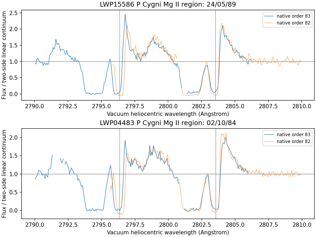
For magnesium, take the median quality-zero flux in 2789–2791 Angstrom from order 83 and in 2808–2810 Angstrom from order 82, then join the two anchors with a straight line. The 1989 anchors contain 30 and 29 samples; the 1984 anchors contain 29 and 29.

This is a reproducible local baseline, not a claim that either window reveals an immaculate stellar continuum. Line blanketing, extraction and calibration may affect it. The first attempt sought both anchors in one order and found no valid red anchor. That failed output and figure are retained; the final calculation explicitly uses the two named orders.

Repeat with a constant baseline equal to the linear baseline at 2799 Angstrom. In some red-component windows the normalized profile changes by about 0.13 continuum units. Report this processing sensitivity separately from independent observations and statistical standard deviations.

Reading: IUE data-analysis FAQ · Standalone stellar-wind scientific reproduction

Plot orders and epochs separately

Run probe-observation.py and inspect both magnesium panels. Each epoch retains orders 83 and 82 as separate curves with their native quality gaps. Do not silently average the overlap.

The two orders come from the same exposure and may share calibration errors. Their disagreement tests robustness; it does not supply two independent repetitions that automatically improve precision. Keeping 1984 and 1989 in separate panels also preserves stellar variability.

The silicon windows are plotted separately. For these more complicated line and absorption structures, the exercise identifies candidate lines and inspects baselines. A quantitative fit would need a richer transfer model.

Separate native orders and quality gaps around magnesium in the 1989 and 1984P Cygni spectra — Flux plotted against vacuum heliocentric wavelength is divided by the local baseline through the two stated anchors. Colors retain orders 83/82; separate panels retain the two epochs.

python3 probe-observation.py --inputs input --out-dir rerun

Reading: IUE NEWSIPS manual, high-dispersion MXHI format · Standalone stellar-wind scientific reproduction

Recompute a conditional isolated-line reference

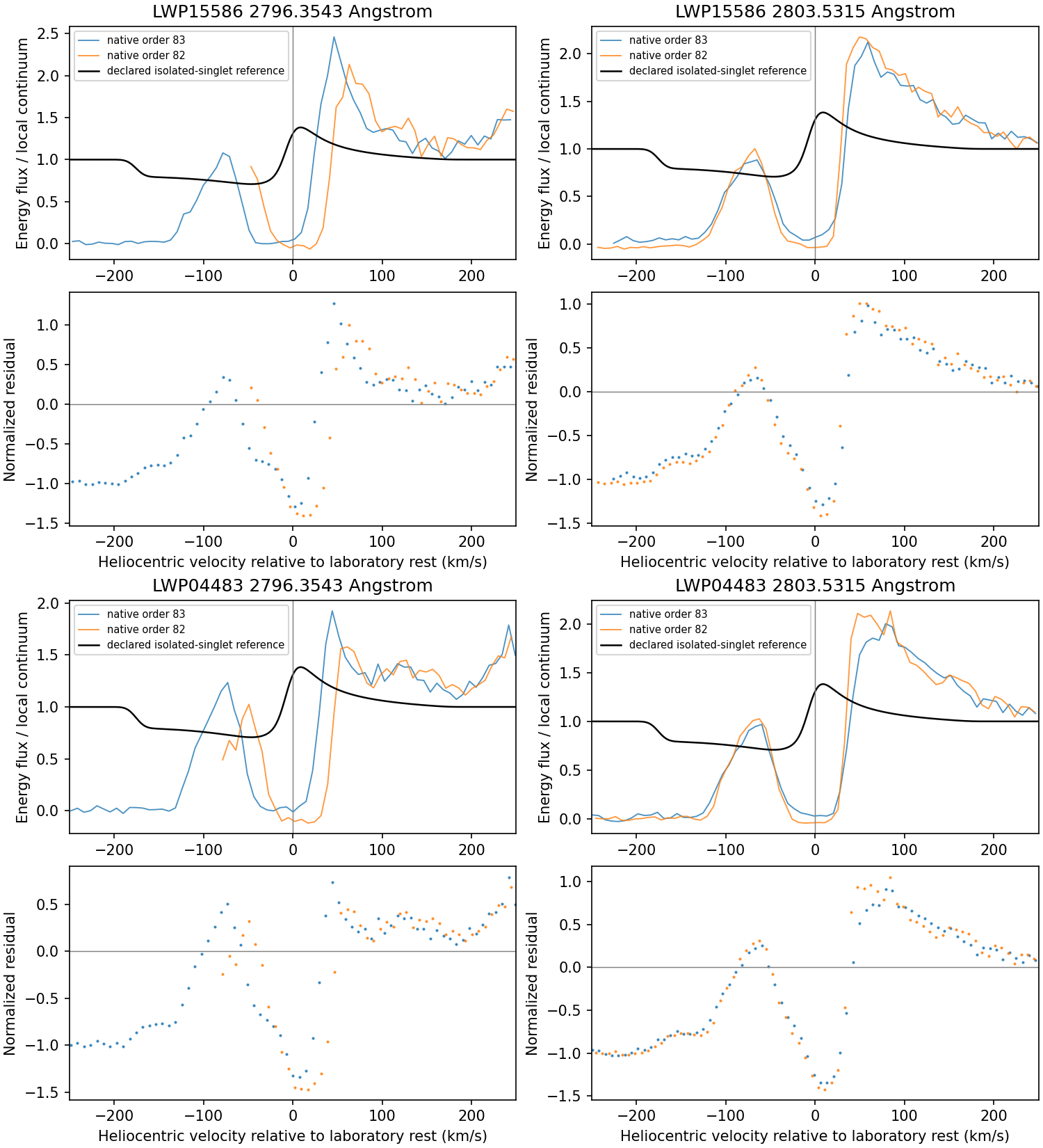
compare_real_line_shapes.py computes an isolated singlet with asymptotic speed 200 kilometres per second, velocity exponent one, product parameter one, full aperture and illustrative instrumental standard deviation 8 kilometres per second. That width was not calibrated from IUE. No parameter optimization makes this a reported best fit.

Compare each magnesium component in its own window extending 250 kilometres per second either side of the laboratory reference. We do not add two isolated-line profiles and call the sum doublet transfer. The reference wind reaches 176.25 kilometres per second at its finite outer boundary; the stated window and width keep its reference components isolated. Blends in the real observation can remain.

Converting an energy spectrum into photons per velocity interval introduces a wavelength factor and the coordinate Jacobian. If the measured flux and local continuum are converted consistently, these factors cancel in their ratio. This permits a normalized-profile comparison while preserving the physical distinction between a structured stellar continuum and the model’s flat illumination.

The program saves eight epoch/order/component comparisons. For the 1989 blue component in order 83, the normalized RMS residual is about 0.66: this ideal reference describes the observed shape poorly. Its residuals can help locate missing photospheric background, interstellar absorption, ion populations, systemic velocity or instrumental effects. They are not a chi-square statistic or a mass-loss uncertainty.

Conditional isolated-line comparisons and residuals for the two P Cygni magnesium epochs — Native orders remain separate above the residual panels. Black curves are the reference under the declared conditions. No calibrated physical noise standard deviation or real mass-loss posterior is assigned.

python3 compare_real_line_shapes.py --inputs input --out-dir rerun

Reading: Standalone stellar-wind scientific reproduction · Lamers, Cerruti-Sola & Perinotto1987, the SEI line-profile method

Why the synthetic count intervals do not transfer

The previous chapter had saved integer photons, a known continuum and instrument, fixed geometry and independent priors from 0.5 to 2 for the mass-flow and ionization multipliers. Even under those conditions a single line identifies their product.

In three fixed-truth experiments with 100 records each, the mass-flow intervals covered 100, 100 and 0 times. In the last case a truth near the prior boundary is repeatedly excluded by the central interval along a broad degeneracy ridge. Interpret that failure alongside prior-averaged coverage. A prior-shaped broad interval is not a precise measurement of mass loss.

The IUE products do not directly supply even the physical count-error model of that synthetic exercise. Retain their calibrated energy flux and FN noise identities. The reproducible work supported here is a comparison of shapes, native orders and continuum sensitivity.

Reading: Standalone stellar-wind scientific reproduction · IUE NEWSIPS manual, high-dispersion MXHI format

Leave a route another reader can replay

Extract into an empty directory, install the pinned NumPy, SciPy and Matplotlib requirements, then run replay.py. It checks input bytes and hashes before actually recomputing transfer, photon fates, force diagnostics, count inference, IUE profiles and the published-table comparison. A receipt is written only after all required steps succeed.

Carry five questions to another spectrum: which wavelength frame, which quality selection, which noise units, which continuum and which fixed physical assumptions? Each answer should point to a saved field or a computation that someone else can inspect.

Reading: Standalone stellar-wind scientific reproduction · MAST original mission data use

Exercises and explanations

What happens if STARTPIX is treated as zero-based?
Read the explanation
Every extracted wavelength shifts by one DELTAW increment. After conversion to velocity, that becomes a systematic displacement that can resemble line structure.
Why not use FN noise as the ABS_CAL uncertainty to compute a chi-square?
Read the explanation
The vectors belong to different calibration stages and units. FN has not undergone the complete conversion needed to become a physical flux standard deviation. Incorrect weights would change the fit and its intervals.
What should a large conditional shape residual prompt first?
Read the explanation
Check the wavelength frame, quality gaps, overlapping orders, continuum and fixed instrumental and physical conditions. Then locate missing backgrounds or blends. A mass-loss inference would additionally need a suitable measurement and uncertainty model.

Try the prediction

Change the flow and follow its scattered light

Switch between the 1989 and 1984 MgII observations without moving model controls; verify that the saved real spectrum stays fixed.
Inspect overlapping orders and gaps, then find the quality selection in the original file rather than interpolating new observations into the gaps.
Replay the independent package. Read a continuum sensitivity result and a conditional residual before naming the next missing calibration or physical ingredient.

Standalone science materials

Download the scientific ZIP · Read the setup and source instructions

The package includes complete small original mission files and licensed published tables. It recomputes transfer, conditional synthetic-count inference and real-data comparisons offline; it does not solve wind acceleration or infer real stellar mass loss.

Sources and calculation scope

Lamers, Cerruti-Sola & Perinotto1987, the SEI line-profile method
ApJ314,726, sectionsII–V and equations4–10/14–19. Our local escape singlet and fixed-source finite-width test retain their separate approximations; no complete SEI/non-LTE solver is claimed.
IUE NEWSIPS manual, high-dispersion MXHI format
Native17-field binary rows, padded768-element vectors, one-based STARTPIX, vacuum heliocentric wavelengths, ABS_CAL physical units and FN noise.
IUE data-analysis FAQ
Questions13–15: reject nonzero quality flags for quantitative use; high-dispersion cosmic rays are not automatically removed; exposure alone does not define a noise weight.
NIST magnesium energy levels
MgII level wavenumbers35760.848/35669.298per centimetre yield laboratory vacuum2796.3543/2803.5315Angstrom. Laboratory rest and stellar systemic velocity are distinct.
MAST original mission data use
Original NASA/ESA/UK IUE public mission products; fixed names, complete bytes and SHA remain in the standalone package with mission/STScI/MAST attribution.
Standalone stellar-wind scientific reproduction
Original small data, independent transfer/photon/force/finite-width references,197producer checks and a proper synthetic Poisson exercise. Fixed truths and prior-averaged coverage remain separate.