Begin with a small velocity perturbation
Open section 2 of the pinned Owocki 2014 v1 review, followed by section 3.1. A steady Sobolev model compresses a narrow resonance region into a local interaction and explains many mean profiles. Line instability instead concerns how a velocity perturbation changes the shadow cast by upstream gas.
If a parcel becomes slightly faster, its Doppler shift changes which stellar frequencies it absorbs. Moving out of a frequency range already depleted upstream can expose it to more direct radiation. The extra acceleration amplifies the perturbation. Scattered diffuse radiation supplies a competing drag, particularly near the photosphere.
The nonlinear calculations in section 3.2 develop compressions, rarefactions and shocks. The Lab’s tracers follow a prescribed steady velocity law. Simulating the formation of such structures would require coupled radiation and gas dynamics, including the shock energy balance.
Reading: Owocki2014, Theory of Winds from Hot, Luminous Massive Stars
Microclumping changes density-squared diagnostics
Consider a volume containing dense and rarefied regions while its mean mass flow remains fixed. The clumping factor compares the mean squared density with the square of the mean. It is at least one, increasing as density fluctuations grow.
In the microclumping limit, clumps are optically thin for the relevant process. With a void interclump medium, the clumping factor is the inverse volume filling fraction. Recombination emission often scales approximately with density squared, so the same mean density produces more emission. Ignoring structure can then attribute that emission to excessive mass loss.
With ionization, emissivity coefficients and geometry held fixed, a fixed recombination signal roughly constrains mass loss times the square root of the clumping factor. This is not a universal correction for every line. Resonance opacity at a fixed ion fraction is first order in density; multiplying it by the same clumping factor is unjustified. In a real atmosphere, structure can also change the ionization balance.
Reading: Owocki2014, Theory of Winds from Hot, Luminous Massive Stars · Brands, Backs, de Koter et al.2025, X-Shooting ULLYSES XII
Thick clumps turn opacity into a coverage problem
Once a clump is optically thick, increasing its internal density need not intercept proportionally more photons. Its projected area, separation, shape and the material between clumps matter. This spatial porosity cannot be replaced by a density-squared multiplier.
A line also selects velocity. At a particular observed frequency, a photon resonates only with material at the appropriate projected speed. If clumps occupy only part of velocity space, gaps let photons through. This velocity porosity, often called vorosity, is distinct from empty space in the geometrical arrangement.
Shallow ultraviolet absorption can therefore reflect low mass flow, fewer relevant ions, incomplete velocity coverage or an interclump medium with its own opacity. Separating these possibilities requires diagnostics with different density and ionization responses and an explicit model of the structure.
Reading: Owocki2014, Theory of Winds from Hot, Luminous Massive Stars · Brands, Backs, de Koter et al.2025, X-Shooting ULLYSES XII
Identify the population in Brands 2025
Next open X-Shooting ULLYSES XII by Brands and colleagues, pinned to arXiv 2503.14687v1. Section 3 describes the FASTWIND 10.6.0 non-LTE atmosphere and wind prescriptions before optical and ultraviolet diagnostics constrain their parameters. A beta velocity law is still prescribed; this is not a radiation-hydrodynamic solution of the acceleration.
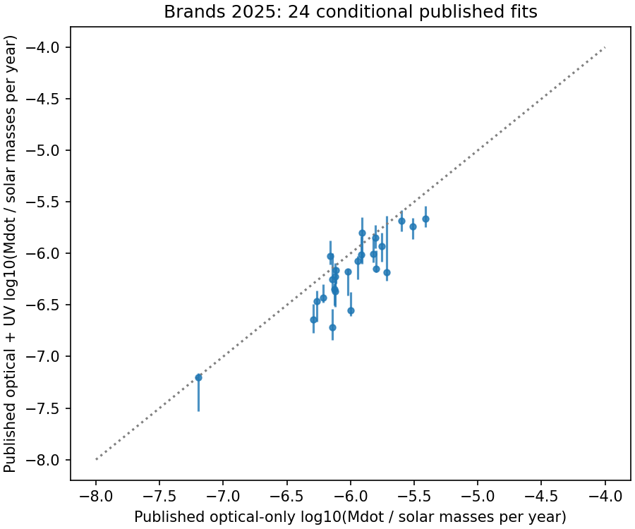
The targets are O-type giants and supergiants in the Large Magellanic Cloud. Twenty-five targets yield 24 parameter sets. They are neither repeated observations of Galactic P Cygni nor 24 independent measurements of the same star. Check Figure 1 and Tables 7/8 before interpreting the between-star trends of section 5.3.
Zenodo record 15044512 version 1.1.1 supplies the complete small optical+UV and optical-only tables and Readme under CC-BY4. Each table has 24 rows. FASTWIND is proprietary, and we did not download the 155 MB model archive. Our replay joins and compares the published table values.
Reading: Brands, Backs, de Koter et al.2025, X-Shooting ULLYSES XII · Brands2025 Zenodo15044512 v1.1.1 tables
Join the two tables by stellar identifier
Run probe-published-fits.py. Read the headers, units and Readme, then match unique target identifiers. The program requires 24 complete pairs and saves each published mass-loss estimate and its change with diagnostic selection. Equal row numbers alone are not a reliable join key.
For these published point estimates, the median optical+UV minus optical-only logarithmic mass-loss difference is about minus 0.1791 dex, corresponding to a ratio near 0.66. It is a descriptive comparison of the 24 pairs: changing the diagnostics can change a conditional inference.
The median does not instruct us to multiply every stellar mass-loss rate by 0.66. Nor are two fits to overlapping data independent experiments whose uncertainties can simply be combined. The point tables lack the full joint likelihood and covariance. Replotting them creates no new physical posterior.
python3 probe-published-fits.py --inputs input --out-dir rerunReading: Brands2025 Zenodo15044512 v1.1.1 tables · Standalone stellar-wind scientific reproduction
Two kinds of correlation answer different questions
Section 5.3 compares stars: across this sample, do stars with a larger value of one parameter tend to have another parameter larger too? Stellar properties, sample selection and modeling assumptions all enter. Such a trend is not an uncertainty ellipse for one star.
Section 5.5 examines parameter degeneracies among fitted models for an individual star. Can a change in clumping or velocity law compensate for higher mass loss while retaining similar fitness? Those interchangeable directions belong to one inference. Calling them a causal stellar-evolution trend changes the statistical object.
Cross-check Figures 4 and 7 against section 5.5. Does a plotted point represent a star, one model, or a sample from a different paper? A 24-row best-fit table cannot reconstruct the authors’ within-star fitness surface. Inspecting that covariance would require the original within-star model ensemble.
Reading: Brands, Backs, de Koter et al.2025, X-Shooting ULLYSES XII
Keep a three-star test within its scope
Section 5.4 refits three stars with optically thin microclumps and a void interclump medium, then compares that prescription with the default treatment allowing optically thick clumps. The authors find best-fit parameters consistent within the uncertainties for these three examples.
That does not establish that every clump is optically thin or that velocity porosity is physically irrelevant. Selected diagnostics can be insensitive to some directions, while other parameters compensate. Preserve the three stars, their diagnostics and the compared model prescriptions when describing the result.
The next useful questions are which lines detect interclump material, which diagnose velocity coverage, and how ionization calculations couple those responses. They lead back to the paper’s evidence more reliably than applying one clumping multiplier to every published mass-loss rate.
Reading: Brands, Backs, de Koter et al.2025, X-Shooting ULLYSES XII