Where the fluid picture of reconnection runs out

Start with a linear perturbation of a specified sheet

Open Loureiro, Schekochihin and Cowley, astro-ph/0703631v1. Follow the equilibrium and matching conditions around equation 3, then the inner/outer matching leading to equation 18. The equilibrium coefficient is determined by the source’s field profile; it is not a freely adjustable transport coefficient.

Keep the full sheet length $L_{\rm CS}$ , its half-thickness $\delta_{\rm CS}$ and the reference flow rate $\Gamma_0$ visible. The dimensionless wave number $\kappa$ measures wavelength along the sheet. The paper’s small-thickness ordering also restricts their product.

The growth rate describes a small perturbation about the assumed sheet. It is not yet a measured nonlinear reconnection rate, a flare duration or the speed at which a magnetic island leaves the layer.

\Gamma_0=\frac{2v_A}{L_{\rm CS}},\quad\kappa=\frac{k v_A}{\Gamma_0},\quad\epsilon=\frac{2\delta_{\rm CS}}{L_{\rm CS}}=\sqrt{\frac{2}{S_{\rm full}}}

The full-length definitions differ from the half-length Lundquist number used in the preceding scaling example.

Sources: Loureiro, Schekochihin & Cowley (2007), astro-ph/0703631v1, equations 3 and 18–20, Figure 4

Read equation 18 and Figure 4 together

Equation 18 is a scalar matching relation involving the Euler gamma function $\Gamma$ . That mathematical function differs from the flow-rate scale $\Gamma_0$ . The reference solves its physical branch with $0<\Lambda<1$ using logarithmic gamma magnitudes and the known sign of the ratio.

The script first determines the equilibrium matching coefficient, about $\alpha=1.30693$ . It then solves the growth relation over wave number and locates its maximum. Repeating the calculation over sheet thickness recovers slopes one quarter for growth and three eighths for the fastest wave number against the full-length Lundquist number.

Look at the vertical ordering limits in the original Figure 4. Our own figure also marks formal continuation outside that range. For $\epsilon=10^{-3}$ , the maximum has $\kappa\epsilon\simeq0.338$ ; for $10^{-6}$ it is about $0.0601$ . A number below one is not automatically asymptotically tiny, so many root digits do not establish comparable physical accuracy.

-\frac\pi8(\kappa\alpha)^{1/3}\Lambda^{5/4}\frac{\Gamma[(\Lambda^{3/2}-1)/4]}{\Gamma[(\Lambda^{3/2}+5)/4]}=\frac{2\alpha^2}{\kappa\epsilon}

The fixed paper’s equation 18. On the selected branch the numerator gamma function is negative, making the complete left side positive.

\frac\gamma{\Gamma_0}=\Lambda\alpha^{2/3}\kappa^{2/3},\qquad\gamma_{\max}/\Gamma_0\propto S_{\rm full}^{1/4},\quad\kappa_{\max}\propto S_{\rm full}^{3/8}

These are linear asymptotic predictions with the equilibrium and ordering attached.

python -W error scripts/astronomy/ac28/run_reference.py
python -W error scripts/astronomy/ac28/test_reference.py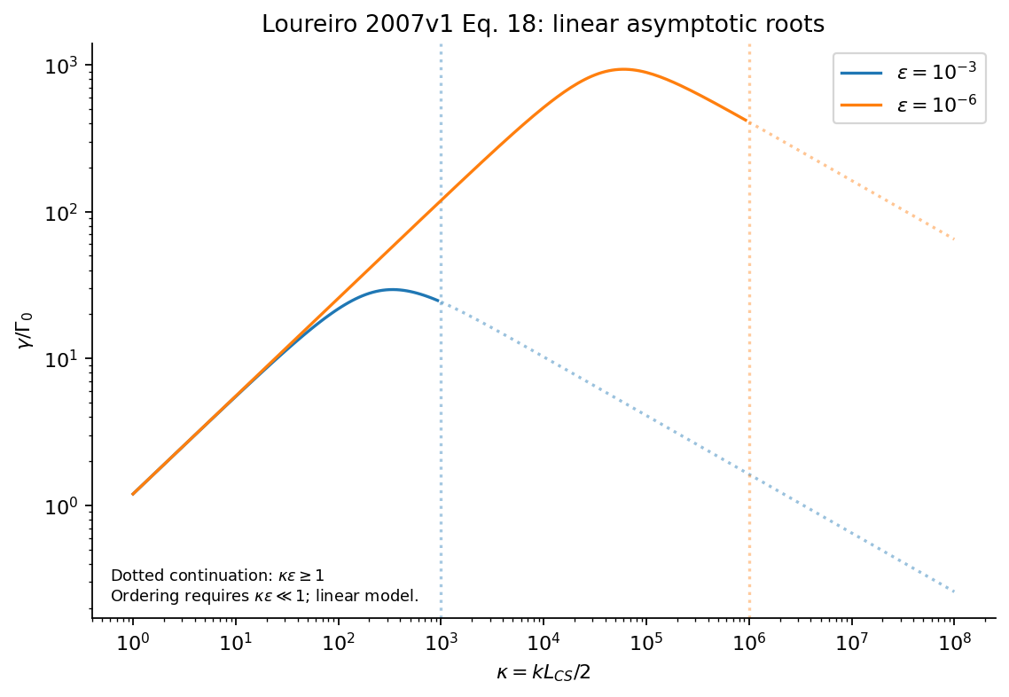

Own numerical roots of the fixed thin-sheet dispersion relation, with ordering-invalid continuation marked. — Recomputed scalar roots of Loureiro 2007v1 equation 18. This calculation produces no nonlinear island evolution.

Sources: Loureiro, Schekochihin & Cowley (2007), astro-ph/0703631v1, equations 3 and 18–20, Figure 4

A nonlinear merger paper asks for a different calculation

Next open Zhou and colleagues, Physical Review Research 1, 012004(R), published in 2019. Equations 1 and 2 describe periodic incompressible reduced MHD. The numerical study begins with an array of magnetic islands, not the two-scale stressed potential used in our small default.

Read Figure 1 first: colour shows current, contours show magnetic flux, and the sequence develops larger structures through mergers. Figure 2 plots total magnetic energy for several initial island-scale Lundquist numbers. Its main time axis is normalized to a reconnection time; the inset uses code time. Mixing those clocks would change the comparison.

The actual grids are $2048^2$ to $8192^2$ , with magnetic Prandtl number one. The studied island-scale Lundquist numbers range from 125 to 1786. The paper states that secondary plasmoids are not expected in these runs and confirms that visually. This is a merger study, not a numerical reproduction of the high-Lundquist plasmoid chain suggested by the first paper.

Figure 3 compares fitted time exponents with the hierarchical model; the later spectrum and scaling discussion tests how power shifts toward larger scales. Read the assumed initial conditions, resolution and fitting interval with those exponents. Reproducing that statistical result requires its multi-island initial condition, resolved evolution and spectral analysis.

Sources: Zhou et al. (2019), Magnetic island merger as a mechanism for inverse magnetic energy transfer, Physical Review Research 1, 012004(R)

Read the electron-scale MMS measurements

Finally open Burch and colleagues, Science 352, aaf2939, published in 2016. The encounter is at Earth’s magnetopause on 16 October 2015. In Figures 3–5, align the electric field, magnetic field, electron velocity and distributions on the reported time axes before interpreting any one panel.

The electron distributions have 30-millisecond cadence. A crescent in velocity space describes how electrons populate different velocities; it is not a physical crescent painted into a plasma image. Connecting a spacecraft time series to spatial structure also requires the boundary motion and crossing geometry.

Compare current estimated from ion/electron moments with current from the multi-spacecraft magnetic curl. The electron-frame nonideal field is $\mathbf E+\mathbf v_e\times\mathbf B$ . Its scalar work diagnostic uses current dotted into that field. A peak in this work quantity does not by itself supply a local entropy-production rate.

Pressure-tensor structure, electron inertia and relative species motion become part of the question at these scales. The scalar collisional closure in the two-dimensional fluid example has no electron distribution to compare with the crescents.

\mathbf J=en(\mathbf v_i-\mathbf v_e),\qquad\mathbf E'_e=\mathbf E+\mathbf v_e\times\mathbf B

Assume approximate quasineutrality and singly charged ions. Here

e

is positive elementary charge and

n

is common number density; the nonrelativistic frame follows electron bulk motion.

D_e=\mathbf J\cdot\mathbf E'_e

This electron-frame field-work diagnostic is distinct from scalar collisional heating and from a measured X-ray intensity.

Sources: Burch et al. (2016), Electron-scale measurements of magnetic reconnection in space, Science 352, aaf2939, Figures 3–5

Build the next physical question from the missing observable

A genuine photospheric-footpoint calculation would prescribe a boundary motion and record the magnetic energy entering through it. A flare-onset study would then need an equilibrium/storage stage and a supported trigger mechanism. Neither can be inferred just by starting an already stressed periodic field.

Predicting X-ray light also requires the emitting plasma and instrument response. Predicting accelerated particles requires distribution or orbit dynamics with a defined energy exchange. Three-dimensional geometry can change field-line connectivity and available modes. Each extension needs new input, a new observable and new validation.

Coronal heating and solar-wind questions can use these distinctions productively: choose the quantity actually measured, identify its source and scale, then ask which model evolves it. The three papers provide a route from a controlled linear sheet to resolved fluid dynamics and finally to electron-scale measurements.

Sources: Loureiro, Schekochihin & Cowley (2007), astro-ph/0703631v1, equations 3 and 18–20, Figure 4 · Zhou et al. (2019), Magnetic island merger as a mechanism for inverse magnetic energy transfer, Physical Review Research 1, 012004(R) · Burch et al. (2016), Electron-scale measurements of magnetic reconnection in space, Science 352, aaf2939, Figures 3–5