Check a Sweet–Parker current sheet against the grid
Sandbox Physics ·
The inflow in one published current sheet agrees with a Sweet–Parker estimate once the calculation’s extra magnetic diffusion is included. Start with three values printed beside the profiles. Then run a separate wave calculation to see how a grid can add diffusion.
Read three cuts through the same current sheet
Open version 3 of Kowal and colleagues’ paper at Figure 7. All three cuts come from one snapshot of a three-dimensional simulation. The boundaries let plasma enter and leave, and the authors selected this snapshot before the turbulent stage.
The top curve is current magnitude across the sheet. Read the separation between its two marked half-height crossings as the plotted thickness δfig. The middle curve gives the inflow vin. The bottom curve gives the outflow vout from a cut along the sheet.
Use the paper’s length convention Lfig=1 throughout this calculation. The setup specifies magnetic diffusivity ηinput=0.001 in the paper’s units. Figure 6 reports a boundary-averaged rate. Keep it separate from the local fits in Figure 7.
The inflow speed times the plotted thickness gives an effective diffusivity of 0.0016256. The excess above the specified value is 0.0006256. Equation 10 offers a separate check from the electric field around a loop. The authors report rough agreement and an HLLD estimate near 0.00061 for this mesh spacing.
The mass-flow estimate gives an outflow of 0.3969. The plotted outflow is 0.387, a 2.49% residual in the flux comparison. The printed intervals allow residuals from −1.22% to 6.15%. The prose reports 0.395 for the outflow. The download preserves that value as a separate calculation.
The explicit diffusivity alone puts the predicted inflow about 22.5% below its fitted value. With the inferred excess included, the difference is 1.25%. This last comparison uses the fitted inflow in the diffusivity estimate, so treat it as a check of consistency.
ηeff≃vinδfig,vinLfig≃voutδfig
The first expression is the paper’s approximate Ohmic balance. The second compares the mass entering and leaving the sheet.
vSP≃ηvout/Lfig
Try the explicit diffusivity first, then the effective value. Use the fitted outflow for both calculations.
A single magnetic wave makes the grid’s contribution measurable. Take one transverse field component in a periodic interval. A prescribed constant speed carries it along, and a specified diffusivity reduces its amplitude.
The finite-volume program starts from cell averages. It advances the cells with a shared flux at each face. The exact continuum wave predicts both phase and amplitude. Fitting the computed amplitude gives an effective diffusivity for this one mode.
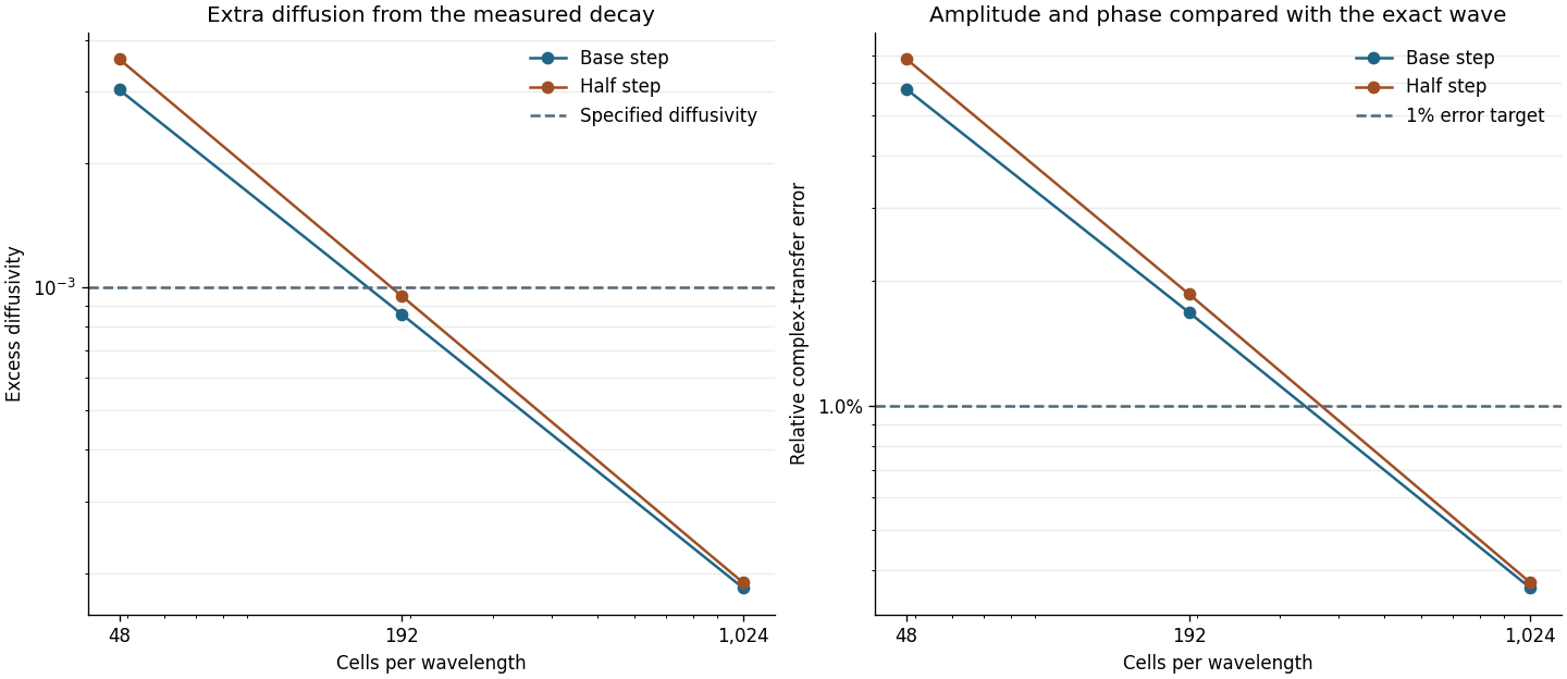
The mean field stays conserved in every run. At 48 cells the amplitude-and-phase error is 5.80%. It falls to 0.36% at 1,024 cells. A held-out wave with nine periods on the 48-cell grid misses the continuum transfer by 99.35%. This run still satisfies the numerical scheme’s discrete Fourier prediction.
∂tB+u∂xB=η∂x2B,ηeff=−k2tln∣Bk(t)/Bk(0)∣
The Fourier coefficient gives the amplitude and phase of the wave at wavenumber k. The absolute value selects the amplitude when estimating diffusion.
The same periodic calculation at three resolutions and two time steps. The 48-cell run adds more diffusion than the specified physical value. The 1% line sets the wave test’s accuracy target.
Check the upstream flow before repeating the estimate
The measured sheet and the wave calculation answer different parts of the problem. The paper’s profiles test a nearly steady inflow and open exhaust. The wave tests numerical attenuation in a simpler system with a known answer. Its fitted diffusivity depends on the grid, timestep, wave and flux rule.
In the magnetic-footpoint Lab, the wall supplies work and the field changes with time. Compare two endpoints at the same model clock. Look at the energy curves before using a steady-layer estimate.
The 48-cell wave conserves its mean field. Why can it still have too much diffusion?
A shared face flux removes exactly what it adds to adjacent cells. Upwind transport still smooths a varying field. The mean can stay fixed as the wave loses amplitude.