Evolve the field and fluid together
Take a periodic square with each side , uniform density and no external driver after the initial state. The invariant direction is . Normalize field by , velocity by and time by . All following equations use these dimensionless coordinates.
The magnetic potential gives the field; a streamfunction gives the incompressible velocity. Current and vorticity use negative Laplacians under this convention. Taking the curl of the momentum equation removes pressure, while solving the streamfunction Poisson relation enforces incompressibility.
The Lorentz-force curl drives vorticity. Fluid advection and magnetic diffusion evolve the potential. Thus the outflow is part of the solution. No independent velocity drawing is added to make a reconnection picture.
Sources: Zhou et al. (2019), Magnetic island merger as a mechanism for inverse magnetic energy transfer, Physical Review Research 1, 012004(R) · Sandbox Physics AC28, independent MHD energy, local-induction and grid/time-reference programs, fixed scientific archive
Derive the energy transfer and its heat terms
Use a domain average to define magnetic and kinetic energy densities. Multiply the potential equation by current and integrate by parts. The magnetic-energy change contains work on the fluid and Ohmic loss. The momentum equation receives the same work with the opposite sign.
Viscosity removes kinetic energy. The symmetric part of the velocity gradient is the strain tensor. In a periodic incompressible plane, its domain-integrated heating equals viscosity times mean vorticity squared. The local maps are different: vorticity squared is not generally the pointwise physical viscous-heating density. The model records only their common domain integral.
Integrating both loss rates with the same Runge–Kutta stages as the fields creates the two dissipative reservoirs. Their sum with field and fluid energy is the unforced model’s check. No conversion from that sum to a solar joule total is possible until a physical volume, including invariant depth, has been specified.
Sources: Zhou et al. (2019), Magnetic island merger as a mechanism for inverse magnetic energy transfer, Physical Review Research 1, 012004(R) · Sandbox Physics AC28, independent MHD energy, local-induction and grid/time-reference programs, fixed scientific archive
Calculate a mode with an answer known in advance
Start with zero fluid motion and a single potential mode . Its current is proportional to its potential, so the magnetic force has zero vorticity source. Only resistive diffusion acts. Solving its scalar time equation gives an exact exponential.
The reference tests amplitude, phase when a uniform mean flow is added, magnetic energy and integrated heat against that answer. It halves the step to measure the fourth-order field error. A separate viscous shear has its own analytic decay. Signed errors are retained; a small negative equivalent numerical diffusivity in this benchmark is a truncation error, not a physical solar transport coefficient.
The nonlinear default supplies an additional sign check. Its initial vorticity acceleration has a known spatial sign and amplitude. Squaring fields to make an energy test would hide a reversal of that force.
Sources: Zhou et al. (2019), Magnetic island merger as a mechanism for inverse magnetic energy transfer, Physical Review Research 1, 012004(R) · Sandbox Physics AC28, independent MHD energy, local-induction and grid/time-reference programs, fixed scientific archive
Compare the actual nonlinear state with a finer grid
The periodic default starts with unequal spatial scales, which leave a nonzero force that the pressure cannot remove completely. At normalized time one, the independent 128-grid solution has the values below. They are rounded for reading; the full-precision JSON is needed to reproduce a tiny energy residual.
At time two, the 128-to 256 current-field relative norm difference is about 0.00436%. The peak-current discrepancy is about 0.00455%. A 64-grid calculation is off by about 2.1% in peak current and a 32-grid calculation by about 20%, even though their global energy sums look excellent.
The four interactive cases also check every saved physical time against the finer grid. Local induction, null identity, field differences and time-step convergence are separate quantities. The fixed parameter cases and endpoints define the tested region.
| At normalized time one | Mean normalized density |
|---|---|
| Magnetic energy | |
| Fluid kinetic energy | |
| Ohmic heat | |
| Viscous heat |
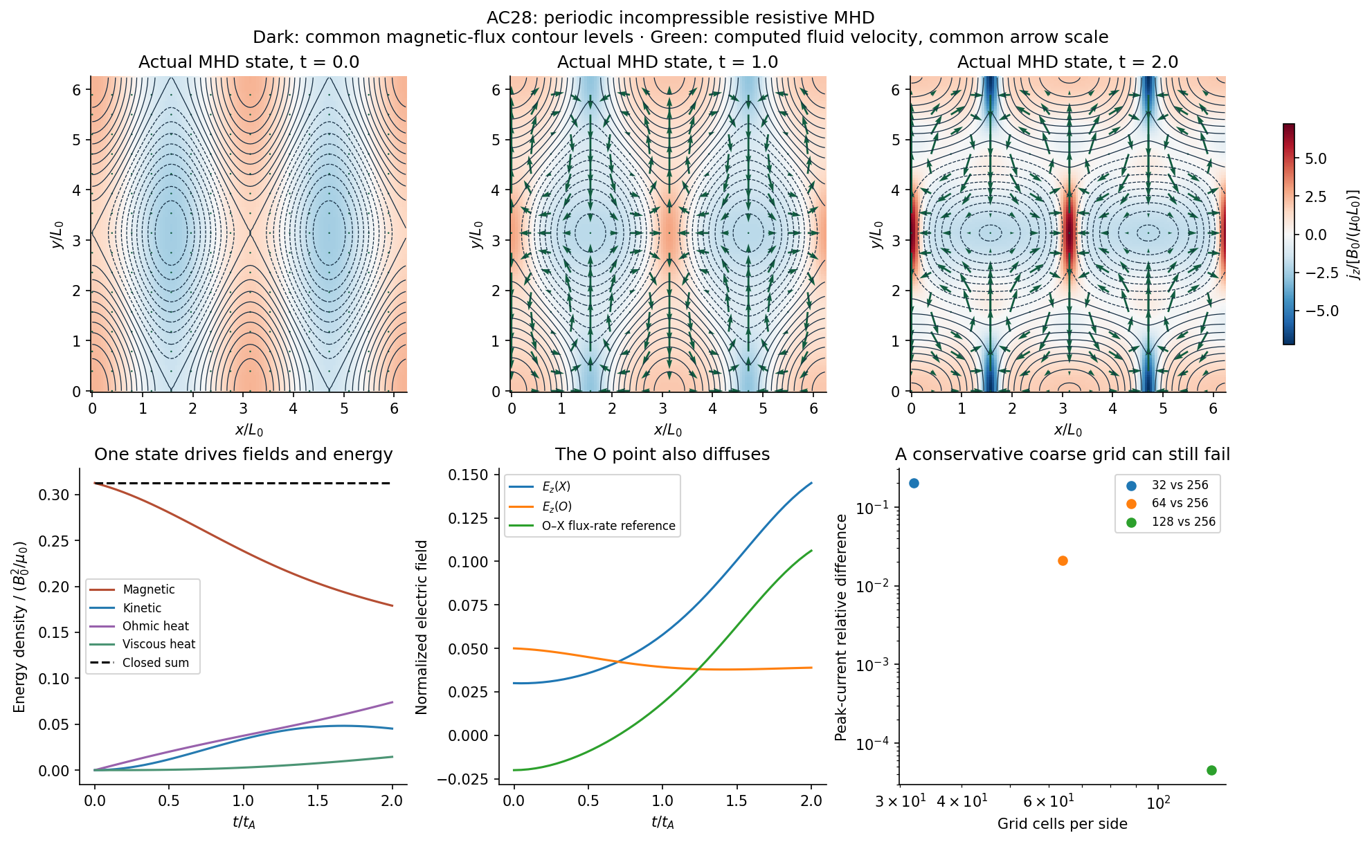
Sources: Zhou et al. (2019), Magnetic island merger as a mechanism for inverse magnetic energy transfer, Physical Review Research 1, 012004(R) · Sandbox Physics AC28, independent MHD energy, local-induction and grid/time-reference programs, fixed scientific archive
A conservative ideal calculation can still change null flux incorrectly
Set both transport coefficients to zero and choose the potentials below. The points and are genuine magnetic nulls. The ideal continuum equation gives zero potential rate at both because its advective term vanishes there.
A Fourier representation adds periodic sine and cosine waves; Galerkin projection returns nonlinear products to the retained wave numbers. Expanding the nonlinear product generates a Fourier harmonic with horizontal wave number sixteen. The 32-grid two-thirds truncation discards it. This removes a cancellation at the nulls, leaving projected rates and . Even an almost empty initial edge-energy spectrum misses the problem.
By time , the coarse O–X contrast has changed about . Energy, mean potential-square and cross-helicity (the mean velocity dotted into magnetic field) still remain at machine-level conservation, and irreversible heat is zero. The same physical initial condition on 64 cells changes the contrast only about .
The failure is a spatial projection error. It must not be relabelled as an extra physical resistivity. This is why the display admits only its tested cases and checks local induction in addition to global invariants.
Sources: Zhou et al. (2019), Magnetic island merger as a mechanism for inverse magnetic energy transfer, Physical Review Research 1, 012004(R) · Sandbox Physics AC28, independent MHD energy, local-induction and grid/time-reference programs, fixed scientific archive
Reproduce the failure and keep both ends of the flux contrast
Unpack the scientific archive and run these commands from its root with the pinned numerical dependencies. The first script regenerates the nonlinear grid/time and analytic checks; the second reruns the retained ideal failure and signed startup. The per-time comparison script compares every saved case/time with the finer solution.
For the closed periodic island, the O point also diffuses. The time derivative of the signed O-minus-X potential therefore uses both electric fields. At the late default state, the finite-grid local induction residual is about seven millionths. The report retains it as a numerical diagnostic, with physical diffusivity fixed at its input value.
python -W error scripts/astronomy/ac28/run_reference.py
python -W error scripts/astronomy/ac28/run_counterexamples.py
python -W error scripts/astronomy/ac28/verify_runtime_domain.py
python -W error scripts/astronomy/ac28/test_reference.py
Sources: Zhou et al. (2019), Magnetic island merger as a mechanism for inverse magnetic energy transfer, Physical Review Research 1, 012004(R) · Sandbox Physics AC28, independent MHD energy, local-induction and grid/time-reference programs, fixed scientific archive