How bubbles appear and fill space

Sandbox Physics · 2026-11-12

A first-order transition finishes when bubbles of the new phase fill space. If the nucleation rate grows exponentially in time with rate $\beta$ , the fraction of space still in the old phase falls as a double exponential, and the bubbles end up spaced by $(8\pi)^{1/3}\xi_w/\beta$ . This chapter derives both results and checks them against a synthetic record of 2803 bubbles.

Units, rate and the old phase

Work in a small region of the universe during the transition, short enough that expansion can be ignored. Time $t$ is measured from a reference time $t_*$ . A bubble that nucleates at time $t'$ grows with constant wall speed $\xi_w$ , in units of the speed of light, so its radius at a later time is $\xi_w(t-t')$ . The old phase is called the false vacuum and the new one the broken phase.

Bubbles can only nucleate where false vacuum is left. Let $\Gamma(t)$ be the number of bubbles nucleated per unit volume and per unit time in false vacuum. Near the end of many thermal transitions this rate rises very steeply, and a good first model is an exponential with rate $\beta$ .

\Gamma(t)=\Gamma_*\,e^{\beta(t-t_*)}

The constant

\Gamma_*

is the rate at the reference time. A larger

\beta

means the transition runs faster. The ratio

\beta/H_*

compares it with the Hubble rate

H_*

at that time; values from ten to a few hundred are typical in the models studied for LISA.

Reading: Caprini et al., Detecting gravitational waves from cosmological phase transitions with LISA: an update, arXiv:1910.13125v2 / JCAP (2020), doi:10.1088/1475-7516/2020/03/024 · Caprini et al., Gravitational waves from first-order phase transitions in LISA: reconstruction pipeline and physics interpretation, arXiv:2403.03723v2 / JCAP 10 (2024) 020

Count how often a point has been swallowed

Pick a point. A bubble born at time $t'$ contains the point at time $t$ if its centre lies within $\xi_w(t-t')$ . Ignore for a moment that later bubbles cannot be born inside earlier ones, and count all "virtual" bubbles. The expected number covering the point is the rate times the volume of that sphere, integrated over birth times.

Bubble centres are scattered at random, so the number of virtual bubbles covering the point follows a Poisson distribution. The point is still in false vacuum only if that number is zero, which has probability $e^{-I}$ . Virtual bubbles born inside real ones would have been inside the broken phase anyway, so they do not change whether the point is covered. That is why the shortcut gives the exact answer for this model.

I(t)=\int_{-\infty}^{t}\Gamma(t')\,\frac{4\pi}{3}\,\xi_w^3(t-t')^3\,dt'=\frac{8\pi\,\xi_w^3\,\Gamma_*}{\beta^4}\,e^{\beta(t-t_*)}

Substitute

s=\beta(t-t')

. The integral becomes

\Gamma_*e^{\beta(t-t_*)}\,(4\pi\xi_w^3/3\beta^4)\int_0^\infty s^3e^{-s}ds

, and the last integral equals

3!=6

h(t)=e^{-I(t)}=\exp\!\left[-e^{\beta(t-t_*)}\right]\quad\text{when}\quad \Gamma_*=\frac{\beta^4}{8\pi\xi_w^3}

Choosing

t_*

so that

I(t_*)=1

fixes

\Gamma_*

. At

t=t_*

about

e^{-1}=37\%

of space is still false vacuum; one unit of

1/\beta

later only

e^{-e}=6.6\%

is left.

From the rate to the bubble spacing

Real bubbles are only born in the false vacuum that is left, so the number density of bubbles at the end is $n_b=\int\Gamma(t)\,h(t)\,dt$ . With $x=\beta(t-t_*)$ the integrand becomes $e^{x}\exp(-e^{x})$ , whose integral over all $x$ is exactly 1. The mean spacing is the cube root of the volume per bubble.

Worked example. Take $\beta/H_*=50$ and $\xi_w=0.9$ . Then $H_*R_*=2.929\times0.9/50=0.0527$ . Bubbles are about five percent of the Hubble radius when they merge. With $\beta/H_*=300$ the same walls give $H_*R_*=0.00879$ .

The LISA template replaces $\xi_w$ by $\max(\xi_w,c_s)$ , where $c_s=1/\sqrt3$ is the sound speed of a relativistic plasma. For slow walls the fluid disturbance runs ahead at nearly sound speed, so the sound speed sets the relevant length.

n_b=\frac{\Gamma_*}{\beta}=\frac{\beta^3}{8\pi\xi_w^3},\qquad R_*=n_b^{-1/3}=(8\pi)^{1/3}\,\frac{\xi_w}{\beta}

This is the mean bubble separation used in the template. Its prefactor

(8\pi)^{1/3}=2.93

comes straight from the exponential rate; a different rate history would change it.

Check it on a synthetic record

We generated one random realisation of this process offline, in a periodic box 40 units of $\xi_w/\beta$ on a side, with seed 77. Bubbles are proposed with the rate above everywhere and kept only when their centre is still in false vacuum. The record keeps the 517 bubbles that cross the displayed slice.

The box should hold $40^3/8\pi=2546$ bubbles on average. This realisation has 2803, ten percent more. That is not a bug: a few early bubbles grow very large, and whether one of them lands in the box changes the count. Over eight seeds the mean ratio is $0.984\pm0.036$ , consistent with 1.

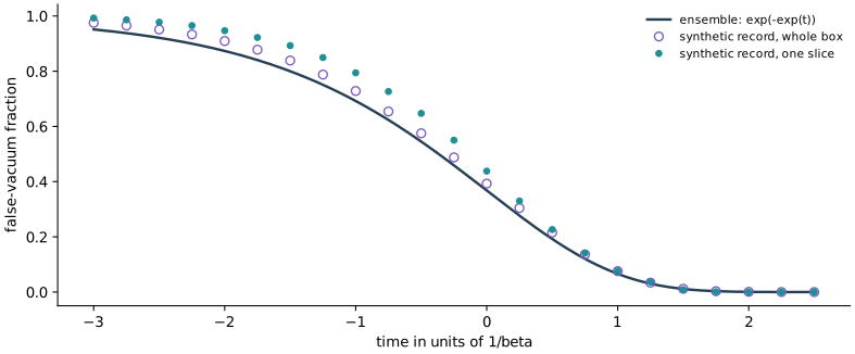
The measured false-vacuum fraction of the whole box stays within 0.039 of $h(t)$ at every sampled time. The fraction measured on the single slice scatters more, up to 0.103, because a slice samples fewer independent bubbles. The Lab plots both, labelled as synthetic, beside the analytic curve.

False-vacuum fraction against time for one synthetic bubble record and the ensemble expectation — One synthetic Monte Carlo record (seed $77$ , $2803$ bubbles in a periodic box of side $40\,v_w/\beta$ ). Open circles count the whole box, filled circles one slice. The line is the ensemble expectation $\exp[-e^{\beta(t-t_*)}]$ for an exponential nucleation rate and a constant wall speed. Open the full figure

Reading: Original benchmark tutorial materials (standard-library Python) · Caprini et al., Detecting gravitational waves from cosmological phase transitions with LISA: an update, arXiv:1910.13125v2 / JCAP (2020), doi:10.1088/1475-7516/2020/03/024

Exercises and explained answers

At what time $\beta(t-t_*)$ is exactly half of space still false vacuum?
Read the explanation
Set $\exp(-e^{x})=1/2$ , so $e^{x}=\ln2$ and $x=\ln(\ln2)=-0.367$ . Half the volume converts a little before the reference time. The steepness of the double exponential means the rest goes within about two units of $1/\beta$ .
Walls move at $\xi_w=0.4$ and $\beta/H_*=100$ . Find $H_*R_*$ with the template rule, and explain why it is larger than $(8\pi)^{1/3}\times0.4/100$ .
Read the explanation
The wall is slower than sound, so the rule uses $c_s=0.577$ : $H_*R_*=2.929\times0.577/100=0.0169$ . The naive value with $0.4$ would be $0.0117$ . For a slow wall, the plasma disturbance it pushes ahead moves near the sound speed, and that disturbance is what sets the sound-wave pattern.
A friend runs the Monte Carlo with one seed and gets 15 percent more bubbles than expected. Is the nucleation code wrong?
Read the explanation
Not necessarily. Bubbles born early grow to sizes comparable to the box, so a single box contains few independent "large" events and its count fluctuates more than a simple square-root estimate suggests. Test the code with an ensemble of seeds and compare the mean, as done here, and compare the volume fraction with $h(t)$ .

Try the prediction

Scrub the tracer bubble through the transition

Predict: in the fraction plot, where should the teal slice points cross one half? Then watch the default run.
Drag the gold handle on the tracer bubble to scrub back to $\beta(t-t_*)=-1$ and count roughly what share of the slice is still purple.
Change $\beta/H_*$ from 50 to 300. The scale bar shrinks: the same picture now spans a much smaller part of the Hubble radius.

Sources and calculation scope

Caprini et al., Gravitational waves from first-order phase transitions in LISA: reconstruction pipeline and physics interpretation, arXiv:2403.03723v2 / JCAP 10 (2024) 020
Read in the arXiv v2 LaTeX source: abstract and introduction, section 2.2.1 (sound-wave double broken power law, amplitude, mean bubble separation and redshift factors), section 3 and appendix A (two-parameter LISA noise and response) and the opening of section 5 on reconstruction. The noise equation prints the optical-metrology corner as 2e-3 mHz; our materials use 2 mHz and report both results. Figure 2 was read from its caption only.
Caprini et al., Detecting gravitational waves from cosmological phase transitions with LISA: an update, arXiv:1910.13125v2 / JCAP (2020), doi:10.1088/1475-7516/2020/03/024
Read the LaTeX source in two places: the sound-wave signal section (signal.tex, about lines 180 to 260) and the definition of the root-mean-square fluid velocity and kinetic-energy fraction (prelim.tex, lines 171 to 182). Used for the earlier shock-time definition only.
Original benchmark tutorial materials (standard-library Python)
Our script, three fixed benchmarks, four failure cases and the expected output. It evaluates the published parametric template, the efficiency fits and the noise model; it does not solve the Einstein or fluid equations and contains no browser Engine code, paper text or LISA data.

Keep reading

What this page links to directly

You are hereHow bubbles appear and fill space

Experiments

Used in this articlePhase-Transition Gravitational Waves from Bubble Collisions

Articles

Phase-transition gravitational waves · Reading path