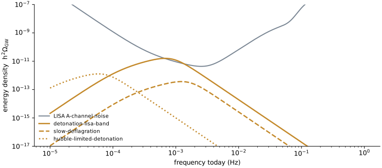
From the sound lifetime to the spectrum today

Sandbox Physics · 2026-11-12

The sound-wave spectrum is fixed by four numbers: the kinetic fraction $K$ , the bubble size $H_*R_*$ , the wall speed and the temperature. For the benchmark $\alpha=0.2$ , $\beta/H_*=50$ , $\xi_w=0.9$ , $T_*=200\,\mathrm{GeV}$ , sound lasts $0.368$ Hubble times before shocks form, and the spectrum today peaks at $h^2\Omega=1.60\times10^{-11}$ near $0.677\,\mathrm{mHz}$ .

How long the sound lasts

Sound waves of amplitude $\bar v_f$ steepen into shocks after about the time it takes the fluid to move one wavelength. The wavelength is set by the bubble size, so the shock-formation time is $\tau_{\rm sh}\sim R_*/\bar v_f$ . After that, the flow turns into shocks and turbulence and the template stops counting it as sound.

The 2024 template uses $\bar v_f^2=K/\Gamma$ , with adiabatic index $\Gamma=4/3$ for radiation, and caps the duration at one Hubble time because expansion dilutes the source after that.

Worked example. $K=0.0274$ gives $\bar v_f=\sqrt{0.0274\times3/4}=0.143$ . With $H_*R_*=0.0527$ , $H_*\tau_{\rm sh}=0.368$ . The sound breaks up after about a third of a Hubble time. For the weak benchmark with $\alpha=0.05$ and $\beta/H_*=10$ , $H_*\tau_{\rm sh}=7.1$ , and the cap of 1 applies.

H_*\tau_{\rm sw}=\min\!\left[\frac{H_*R_*}{\sqrt{K/\Gamma}},\,1\right]

Ellis, Lewicki and No (2020) argued that for many models the first entry is smaller than 1. Guo, Sinha, Vagie and White (2021) instead derived a smooth suppression factor

\Upsilon=1-1/\sqrt{1+2H_*\tau_{\rm sh}}

for radiation domination; for the benchmark it gives

0.241

instead of

0.368

. The Lab plots both, and uses the minimum rule because the template was calibrated with it.

Reading: Caprini et al., Gravitational waves from first-order phase transitions in LISA: reconstruction pipeline and physics interpretation, arXiv:2403.03723v2 / JCAP 10 (2024) 020 · Ellis, Lewicki & No, Gravitational waves from first-order cosmological phase transitions: lifetime of the sound wave source, arXiv:2003.07360v4 / JCAP 07 (2020) 050

The shape: a double broken power law

The spectrum rises as $f^3$ at low frequency, runs as $f^1$ between two breaks and falls as $f^{-3}$ above the second; the 2024 paper takes these exponents from fluid simulations. The first break is set by the bubble size and the second by the sound-shell thickness, so both scale as $1/R_*$ .

The integrated amplitude $\Omega_{\rm int}$ is the spectrum integrated over $\ln f$ . It grows as $K^2$ , with the source duration and with the bubble size. The constant $A_{\rm sw}=0.11$ is an average over simulations at different $\alpha$ and $\xi_w$ .

We checked the normalisation independently. Integrating the shape numerically over $\ln f$ for the benchmark ratio $f_2/f_1=6.97$ reproduces the printed relation between $\Omega_2$ , the amplitude at the second break, and $\Omega_{\rm int}$ to better than one part in a million, and gives $\Omega_2/\Omega_{\rm int}=0.540$ .

h^2\Omega_{\rm int}=h^2F_{\rm GW,0}\,A_{\rm sw}\,K^2\,(H_*\tau_{\rm sw})(H_*R_*),\qquad f_1\simeq\frac{0.2\,H_{*,0}}{H_*R_*},\qquad f_2\simeq\frac{0.5\,H_{*,0}}{\Delta_w\,H_*R_*}

Here

\Delta_w=\xi_{\rm shell}/\max(\xi_w,c_s)

. For the benchmark

\Delta_w=(0.9-0.577)/0.9=0.358

. The constants

F_{\rm GW,0}

and

H_{*,0}

carry the redshift and are derived in the next section.

\Omega_2=\frac{1}{\pi}\left(\sqrt2+\frac{2f_2/f_1}{1+f_2^2/f_1^2}\right)\Omega_{\rm int}

Equation Om2_sound of arXiv:2403.03723v2. The paper quotes

\approx0.55

for

\xi_w\approx1

; at

\xi_w=0.9

the ratio is 0.540.

Sound-wave template spectra today for three fixed benchmarks with the LISA noise curve — Template spectra $h^2\Omega_{\mathrm{GW}}(f)$ today for the three tutorial benchmarks, computed by the tutorial script. Grey is the LISA noise written as an energy density, with the optical-metrology corner at $2\,\mathrm{mHz}$ . These are evaluations of a parametric template, not simulations or measured data. Open the full figure

Reading: Caprini et al., Gravitational waves from first-order phase transitions in LISA: reconstruction pipeline and physics interpretation, arXiv:2403.03723v2 / JCAP 10 (2024) 020 · Caprini et al., Detecting gravitational waves from cosmological phase transitions with LISA: an update, arXiv:1910.13125v2 / JCAP (2020), doi:10.1088/1475-7516/2020/03/024

Redshift to today from first principles

A wave produced with frequency $f_*$ is observed today at $f=f_*\,a_*/a_0$ . Entropy per comoving volume is conserved, so $g_{s}a^3T^3$ is constant, giving $a_*/a_0=(g_{s,0}/g_{s,*})^{1/3}\,T_0/T_*$ with $g_{s,0}=3.909$ and CMB temperature $T_0=2.7255\,\mathrm{K}$ . The Hubble rate during radiation domination follows from the Friedmann equation.

Multiplying gives $H_{*,0}$ . Our own evaluation with these constants gives $1.6467\times10^{-5}\,\mathrm{Hz}$ at $100\,\mathrm{GeV}$ and $g_*=100$ , within 0.2 percent of the printed $1.65\times10^{-5}$ . The energy density of radiation falls as $a^{-4}$ while the critical density falls as $H^2$ ; the ratio gives $h^2F_{\rm GW,0}=1.6404\times10^{-5}$ , against the printed $1.64\times10^{-5}$ .

Putting the benchmark together: $H_{*,0}=3.30\times10^{-5}\,\mathrm{Hz}$ at 200 GeV, $f_1=0.125\,\mathrm{mHz}$ , $f_2=0.873\,\mathrm{mHz}$ , $h^2\Omega_{\rm int}=2.63\times10^{-11}$ , and a peak of $1.60\times10^{-11}$ at $0.677\,\mathrm{mHz}$ .

H_*=\sqrt{\frac{8\pi^3g_*}{90}}\,\frac{T_*^2}{M_{\rm Pl}},\qquad H_{*,0}=\frac{a_*}{a_0}H_*\simeq1.65\times10^{-5}\,\mathrm{Hz}\left(\frac{g_*}{100}\right)^{1/6}\frac{T_*}{100\,\mathrm{GeV}}

M_{\rm Pl}=1.22\times10^{19}\,\mathrm{GeV}

is the Planck mass. We assume

g_{s,*}=g_*

, as the template does. Temperature only shifts the spectrum in frequency; it does not change

h^2\Omega

at fixed

g_*

Can LISA hear it?

The template is compared with LISA noise expressed in the same units. We use the two-parameter noise model of the 2024 paper: test-mass acceleration noise $3\times10^{-15}\,\mathrm{m\,s^{-2}\,Hz^{-1/2}}$ and optical metrology noise $15\times10^{-12}\,\mathrm{m\,Hz^{-1/2}}$ , in the A and E channels. No galactic or extragalactic foreground is included.

The signal-to-noise ratio for four years of data is $\mathrm{SNR}=\sqrt{2T\int(\Omega/\Omega_N)^2df}$ , with the factor 2 for the two channels. The benchmark gives 634, the slow-wall benchmark 33.7 and the Hubble-limited weak transition 0.20.

As an independent check of the noise curve, the sky-averaged sensitivity of Robson, Cornish and Liu should exceed our single-channel curve by a factor tending to $20/9$ at low frequency, because their curve uses a sky-averaged response and a different normalisation. Our numbers reproduce that limit, which checks the units and the low-frequency acceleration term.

Reading: Caprini et al., Gravitational waves from first-order phase transitions in LISA: reconstruction pipeline and physics interpretation, arXiv:2403.03723v2 / JCAP 10 (2024) 020 · Robson, Cornish & Liu, The construction and use of LISA sensitivity curves, arXiv:1803.01944v2 / Class. Quantum Grav. (2019), doi:10.1088/1361-6382/ab1101

Exercises and explained answers

Keep everything in the benchmark fixed but raise the temperature to 1 TeV. What happens to $f_1$ , $f_2$ and the peak height?
Read the explanation
Both breaks scale with $H_{*,0}\propto T_*$ , so they move up by a factor 5: $f_1=0.626\,\mathrm{mHz}$ , $f_2=4.36\,\mathrm{mHz}$ . The height $h^2\Omega$ is unchanged at fixed $g_*$ , because $F_{\rm GW,0}$ depends only on $g_*$ .
For the weak benchmark, $H_*\tau_{\rm sh}=7.1$ . Why does the template use 1 instead, and what would the amplitude be without the cap?
Read the explanation
After about one Hubble time, expansion has diluted the source and the sound waves no longer add coherently to the gravitational-wave energy at the same rate. Without the cap the amplitude would be 7.1 times larger. The smooth factor $\Upsilon=0.744$ of Guo et al. gives a value between the two estimates.
Ellis, Lewicki and No use $\bar U_f^2=\tfrac34\kappa\alpha/(1+\alpha)$ . Compute $H_*\tau_{\rm sh}$ for the benchmark with that definition and compare.
Read the explanation
$\kappa\alpha/(1+\alpha)=0.0457$ , so $\bar U_f=\sqrt{0.0343}=0.185$ and $H_*\tau_{\rm sh}=0.0527/0.185=0.285$ , against $0.368$ with the 2024 definition. The difference is the factor 0.6 in $K$ . Two papers that agree on the physics still give source lifetimes that differ by 30 percent here.

Try the prediction

Compare the two sound-lifetime rules

Predict which way the peak moves when the temperature is raised to 1 TeV in the advanced panel, then try it.
Choose the preset Sound outlasts a Hubble time and compare the two lifetime rules in the lifetime plot.
Choose Strong, sound breaks up fast and note how far below 1 the sound lifetime falls.

Sources and calculation scope

Caprini et al., Gravitational waves from first-order phase transitions in LISA: reconstruction pipeline and physics interpretation, arXiv:2403.03723v2 / JCAP 10 (2024) 020
Read in the arXiv v2 LaTeX source: abstract and introduction, section 2.2.1 (sound-wave double broken power law, amplitude, mean bubble separation and redshift factors), section 3 and appendix A (two-parameter LISA noise and response) and the opening of section 5 on reconstruction. The noise equation prints the optical-metrology corner as 2e-3 mHz; our materials use 2 mHz and report both results. Figure 2 was read from its caption only.
Caprini et al., Detecting gravitational waves from cosmological phase transitions with LISA: an update, arXiv:1910.13125v2 / JCAP (2020), doi:10.1088/1475-7516/2020/03/024
Read the LaTeX source in two places: the sound-wave signal section (signal.tex, about lines 180 to 260) and the definition of the root-mean-square fluid velocity and kinetic-energy fraction (prelim.tex, lines 171 to 182). Used for the earlier shock-time definition only.
Ellis, Lewicki & No, Gravitational waves from first-order cosmological phase transitions: lifetime of the sound wave source, arXiv:2003.07360v4 / JCAP 07 (2020) 050
Read the LaTeX source for the shock-formation time, the mean fluid velocity written through the efficiency, and the argument that the sound-wave source switches off well before a Hubble time for strong transitions.
Robson, Cornish & Liu, The construction and use of LISA sensitivity curves, arXiv:1803.01944v2 / Class. Quantum Grav. (2019), doi:10.1088/1361-6382/ab1101
Located the optical-metrology and test-mass noise terms and the sensitivity formula in the LaTeX source. Used only as an independent check of the noise curve shape and of the 2 mHz corner; the paper was not read section by section.
Original benchmark tutorial materials (standard-library Python)
Our script, three fixed benchmarks, four failure cases and the expected output. It evaluates the published parametric template, the efficiency fits and the noise model; it does not solve the Einstein or fluid equations and contains no browser Engine code, paper text or LISA data.

Keep reading

What this page links to directly

You are hereFrom the sound lifetime to the spectrum today

Experiments

Used in this articlePhase-Transition Gravitational Waves from Bubble Collisions

Articles

Phase-transition gravitational waves · Reading path