Read the LISA sound-wave template and its limits

What kind of claim each source makes

All five papers used in this course are published in journals: arXiv:2403.03723 in JCAP 2024, arXiv:2003.07360 in JCAP 2020, arXiv:2007.08537 in JCAP 2021, arXiv:1910.13125 in JCAP 2020 and arXiv:1004.4187 in JCAP 2010. We read the arXiv versions named here, not the journal typesetting. None of them reports an observation: no phase-transition background has been detected.

Their content is of three kinds. Fits to fluid simulations, such as the slopes and the constant $A_{\rm sw}$, are numerical results within the simulated range. The template, the lifetime rule and the LISA forecasts are model predictions. Questions the papers raise but do not settle, such as the spectrum near the Jouguet speed or after shocks form, are open problems. Our own Monte Carlo record and profile solutions are synthetic calculations made for this course.

Reading: Caprini et al., Gravitational waves from first-order phase transitions in LISA: reconstruction pipeline and physics interpretation, arXiv:2403.03723v2 / JCAP 10 (2024) 020 · Ellis, Lewicki & No, Gravitational waves from first-order cosmological phase transitions: lifetime of the sound wave source, arXiv:2003.07360v4 / JCAP 07 (2020) 050 · Guo, Sinha, Vagie & White, Phase transitions in an expanding universe: stochastic gravitational waves in standard and non-standard histories, arXiv:2007.08537v3 / JCAP 01 (2021) 001 · Caprini et al., Detecting gravitational waves from cosmological phase transitions with LISA: an update, arXiv:1910.13125v2 / JCAP (2020), doi:10.1088/1475-7516/2020/03/024

Section 2.2.1: read each symbol before the equations

The section opens with the physical picture: bulk fluid motion is mostly compressional at first, and after collisions the compression waves source gravitational waves. It then cites lattice simulations and the "Higgsless" approach, which replaces the scalar field by a prescribed, expanding true-vacuum background so that the fluid and its shocks can be solved accurately.

Equations sw_shape, sw_amplitude and Rstar define the template. Read $\Delta_w=\xi_{\rm shell}/\max(\xi_w,c_s)$ carefully: the text says $\xi_{\rm shell}=|\xi_w-c_s|$ holds for subsonic deflagrations and detonations, "the cases we focus on in this work, as we set $\xi_w$ close to unity". A reader who plugs a hybrid wall into the same formula is outside what the authors state.

The kinetic fraction is $K\simeq0.6\,\kappa\alpha/(1+\alpha)$. The factor 0.6 comes from many-bubble simulations and is called a conservative estimate compared with the 2020 review, which used $K=\kappa\alpha/(1+\alpha)$. Common misreading: comparing amplitudes from the two papers at the same $\alpha$ and $\xi_w$ without noticing that $K^2$ differs by a factor 0.36.

Reading: Caprini et al., Gravitational waves from first-order phase transitions in LISA: reconstruction pipeline and physics interpretation, arXiv:2403.03723v2 / JCAP 10 (2024) 020 · Espinosa, Konstandin, No & Servant, Energy budget of cosmological first-order phase transitions, arXiv:1004.4187v1 / JCAP 1006:028 (2010)

The sound-wave panel of the parameter figure

Find the panel labelled fig:pars_PT_sw in the source, the second panel of the parameter-dependence figure. Its caption fixes the black reference spectrum at $K=0.1$, $H_*R_*=0.1$, $\xi_w=0.9$ and $T_*=1\,\mathrm{TeV}$; each coloured line varies one parameter, and the dashed grey line is the LISA noise.

We read the caption and the equations, not the plotted pixels. From the equations you can predict what each family of lines must do, and then check it in the figure. Changing $T_*$ shifts the curve sideways without changing its height. Changing $\xi_w$ moves only the second break, through $\Delta_w$. Changing $H_*R_*$ moves both breaks and also changes the height, because both $H_*R_*$ and the lifetime enter the amplitude. Changing $K$ raises the curve as $K^2$ while the lifetime stays at 1, and more slowly once shocks form first.

The Lab draws the same template and lets you make these one-parameter changes yourself; the gold curve disappears outside the domain of the template.

Reading: Caprini et al., Gravitational waves from first-order phase transitions in LISA: reconstruction pipeline and physics interpretation, arXiv:2403.03723v2 / JCAP 10 (2024) 020 · Original benchmark tutorial materials (standard-library Python)

How long the sound lasts: three versions

Ellis, Lewicki and No (arXiv:2003.07360v4) estimate the shock-formation time as $\tau_{\rm sh}\sim L_f/\bar U_f$, with $\bar U_f^2\simeq\tfrac34\kappa\alpha/(1+\alpha)$. Their abstract argues that in models without a zero-temperature barrier, and in scale-invariant models, sound lasts only a fraction of a Hubble time. The 2020 LISA review reduces the power by $H_*\tau_{\rm sh}=H_*R_*/K^{1/2}$. The 2024 template uses $H_*R_*/\sqrt{K/\Gamma}$ and caps it at 1.

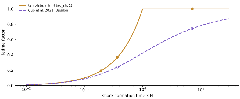
For our benchmark, $\alpha=0.2$, $\beta/H_*=50$, $\xi_w=0.9$, these give $0.285$, $0.247$ and $0.368$. The physics is the same; the definitions of fluid speed differ. Guo, Sinha, Vagie and White (arXiv:2007.08537v3) replace the sharp cap by $\Upsilon=1-1/\sqrt{1+2H_*\tau_{\rm sh}}$ in radiation domination, which gives $0.241$.

What happens to gravitational-wave production after shocks form is not settled in these papers. The 2024 template stops counting the sound and adds turbulence as a separate, uncertain contribution with its own efficiency parameter. The lifetime factor is therefore one of the largest modelling uncertainties in the amplitude.

Reading: Ellis, Lewicki & No, Gravitational waves from first-order cosmological phase transitions: lifetime of the sound wave source, arXiv:2003.07360v4 / JCAP 07 (2020) 050 · Guo, Sinha, Vagie & White, Phase transitions in an expanding universe: stochastic gravitational waves in standard and non-standard histories, arXiv:2007.08537v3 / JCAP 01 (2021) 001 · Caprini et al., Detecting gravitational waves from cosmological phase transitions with LISA: an update, arXiv:1910.13125v2 / JCAP (2020), doi:10.1088/1475-7516/2020/03/024 · Caprini et al., Gravitational waves from first-order phase transitions in LISA: reconstruction pipeline and physics interpretation, arXiv:2403.03723v2 / JCAP 10 (2024) 020

Wall speed is an input, not an output

In every formula here $\xi_w$ is a free parameter. None of the papers we read computes it from the friction between wall and plasma. The 2020 review states that its ansatz is most reliable when the wall speed is far from the Chapman–Jouguet speed: for deflagrations well below $c_s$, for detonations well above it. Near that speed the shells are thin, with thickness about $R_*|\xi_w-c_s|/c_s$, and the spectral shape fails.

This matters for identifiability. If the wall speed of a real transition sits near the sound speed, the template would mismodel the second break, which is exactly the feature that carries $\xi_w$.

Reading: Caprini et al., Detecting gravitational waves from cosmological phase transitions with LISA: an update, arXiv:1910.13125v2 / JCAP (2020), doi:10.1088/1475-7516/2020/03/024 · Caprini et al., Gravitational waves from first-order phase transitions in LISA: reconstruction pipeline and physics interpretation, arXiv:2403.03723v2 / JCAP 10 (2024) 020

Section 5: what LISA could identify

Section 5 of arXiv:2403.03723v2 states the key counting problem. A double broken power law has three geometric parameters, the amplitude and two breaks, while sound waves depend on four thermodynamic ones, $K$, $H_*R_*$, $\xi_w$ and $T_*$. The inversion is therefore degenerate. The authors show the degeneracies can be lifted when more than one contribution is reconstructed, and they reconstruct geometric parameters first and convert afterwards.

Read the limits stated in the abstract and introduction before quoting the forecast of better than about 10 percent accuracy. The simulated data use the same templates for signal, noise and foregrounds as the reconstruction, so template error is absent by construction. General-relativistic effects for bubbles comparable to the Hubble size are neglected, and the noise model has two parameters. The forecast holds "if certain experimental and theoretical uncertainties are solved by the time LISA flies".

Checklist for the next paper in this field: which wall regimes the template covers; which definition of $K$ and of fluid speed it uses; how the lifetime is capped; whether foregrounds are included; whether the injected and fitted templates are the same; which numbers are simulation fits, which are forecasts, and which questions remain open.

Reading: Caprini et al., Gravitational waves from first-order phase transitions in LISA: reconstruction pipeline and physics interpretation, arXiv:2403.03723v2 / JCAP 10 (2024) 020 · Robson, Cornish & Liu, The construction and use of LISA sensitivity curves, arXiv:1803.01944v2 / Class. Quantum Grav. (2019), doi:10.1088/1361-6382/ab1101