Separate expansion from peculiar motion
Keep the observer on the negative side, with positive velocity directed away. Gas recedes with the overall expansion and can also move relative to that flow. The latter is peculiar velocity. In a thin slice at fixed redshift, the sum gives the spectral centre assigned to each comoving location.
Here is the Hubble rate, converts comoving distance to proper distance, and is the peculiar-velocity component along the sightline. Positive peculiar motion shifts absorption redward; a negative component shifts it blueward.
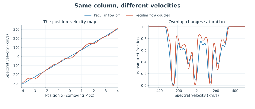
Without peculiar motion, the graph is a straight rising line. With it, the mapping can become shallower, steeper or locally turn back. Its horizontal axis still represents spatial position; its vertical axis is spectral velocity.

Reading: Peeples et al., Pressure Support versus Thermal Broadening in the Lyman-alpha Forest, arXiv:0910.0256v3 · Independent hydrogen and sightline calculation materials
A shallow map gathers more gas
Temporarily use proper distance and examine a monotonic piece of the curve. A narrow velocity interval corresponds to a short path where the curve is steep. The same interval gathers a longer path where it is shallow.
The slope measures how much recession velocity changes per distance travelled. The path contained in a small velocity interval is inversely proportional to the slope’s magnitude. At equal neutral density, the shallower region supplies more column to that interval.
To isolate this weighting, idealize the entire line profile as a spike of vanishing width but fixed area. Both thermal and natural widths are neglected in this mathematical limit. If the selected velocity has several separate spatial crossings with nonzero slopes, add all their contributions.
For a pure Hubble flow, the proper-distance slope is the Hubble rate. Uniform density then recovers the preceding chapter’s uniform Gunn–Peterson relation: the two arguments agree in units and weighting.
Reading: Peeples et al., Pressure Support versus Thermal Broadening in the Lyman-alpha Forest, arXiv:0910.0256v3 · Independent hydrogen and sightline calculation materials
Keep finite width at a fold
At a turning point, the narrow-line denominator approaches zero. The zero-width position-to-velocity weighting diverges there. Finite line width spreads the crowded absorption across a range of velocities. The atoms still have thermal velocities and a natural line width.
The actual calculation walks through space and adds the complete Voigt cross section of each segment. Neighbouring segments may share similar velocities, but they contain finite numbers of atoms and the cross-section peak is finite. Forward integration does not divide by the slope at a fold.
Every spatial location still has one prescribed bulk velocity. The folded graph maps positions into spectral velocities; it does not calculate several fluid streams at one location. The fold itself supplies no evidence for collisions, shocks or evolved gas dynamics.
Reading: Tepper García, Voigt profile fitting to quasar absorption lines, arXiv:astro-ph/0602124v1 · Independent hydrogen and sightline calculation materials
One column can give different mean transmission
Change only peculiar velocity, keeping the sightline, neutral abundance and temperature fixed. Column density stays fixed. Integrating the optical depth over all velocities also preserves its area: motion redistributes the contributions.
Transmission is an exponential of optical depth. Overlapping two contributions can further darken an already dark region while leaving another part of the spectrum free. Equal column therefore does not prescribe equal mean transmission.
For a counting example, use two ideal rectangular lines, each of width and optical depth one. Separated lines have two missing-light areas; overlapping them puts optical depth two inside one width. Their areas below differ even though the optical-depth area is identical. Rectangles are only this arithmetic example, not the hydrogen profile used in the calculation.
The fixed gas screen gives a concrete comparison. Between −500 and +500 kilometres per second, the mean of 601 samples is about 66.8 percent at zero peculiar-velocity strength and 72.6 percent at strength two. Both columns are about . These are prescribed-model results, with a declared velocity window and sampling.
Reading: Independent hydrogen and sightline calculation materials
What is missing when we infer locations from dips?
The forward problem has a clear order: specify gas in space and its motion, then calculate the spectrum. A single dip permits several explanations, including more neutral hydrogen, a shallower velocity map or overlapping contributions. Temperature changes the width of each contribution as well.
Neighbouring sightlines sample different density and velocity combinations. Multiple transitions, statistical distributions and simulations add further information. Each addition must be connected to the particular unknown that it constrains.
Rotating a graph on paper does not change the frequencies already received by a telescope. Fix the physical viewing direction first, then keep spatial position distinct from spectral velocity. Crowding becomes a well-defined physical question.
Reading: Peeples et al., Pressure Support versus Thermal Broadening in the Lyman-alpha Forest, arXiv:0910.0256v3 · Independent hydrogen and sightline calculation materials