The Lyman-alpha forest · L4

Read a thermal history in small-scale velocity gradients

Sandbox Physics · 2026-11-05

Present temperature does not uniquely determine how smooth gas is today. Earlier pressure forces leave a history-dependent response. The July 2026 preprint 2607.19938v1 investigates another trace: how that history affects small-scale velocity gradients and, through them, Ly-alpha flux power. Reading each model conversion makes its fitted scale more informative than treating the final number as a length directly resolved by a telescope.

Why equal temperatures today are insufficient

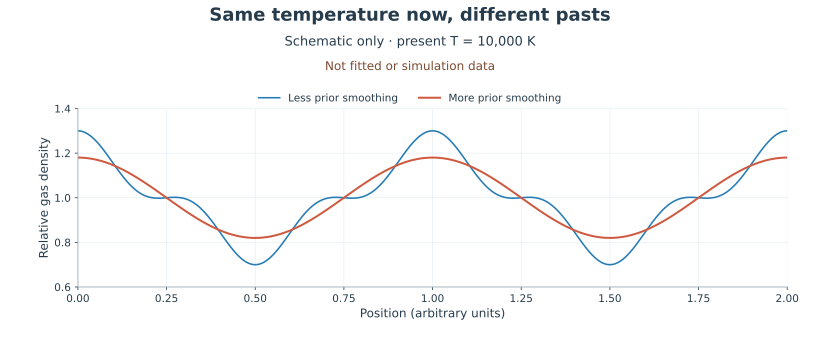
Consider two patches at the same present temperature. One was heated early, leaving pressure more time to redistribute small structures; the other was heated recently. Their instantaneous atomic thermal motions can be similar while their density and bulk-motion structures differ. Current thermal broadening and accumulated pressure response are separate physical effects.

Thermal broadening spreads each location’s absorption across velocity. Pressure smoothing changes how gas has distributed itself and moved. Dark-matter free streaming can also reduce small-scale structure, through a different stage. Early particle motion suppresses small matter perturbations; gas pressure reshapes baryonic structure, while current thermal broadening acts when gas is mapped into a spectrum. All can reduce fine structure in flux; a smoother spectrum alone does not identify which one is responsible.

Peeples and colleagues compared pressure support with thermal broadening and showed how the temperature–density relation affects their relative appearance in longitudinal statistics. The new preprint focuses on a velocity-gradient feature and proposes a bridge to observable flux power. Keep those questions distinct before interpreting a turnover in a plot.

Conceptual structures with the same current temperature but different pressure histories — Original schematic in arbitrary spatial units: longer pressure response can erase smaller structures even at equal present temperature. Curves are conceptual, not hydrodynamic output, a fitted power spectrum or a reproduction of the source paper. Open the full figure

Reading: Peeples et al., Pressure Support versus Thermal Broadening in the Lyman-alpha Forest, arXiv:0910.0256v3 · Iršič et al., Ringing of the Reionization, arXiv:2607.19938v1

Identify the velocity quantity being plotted

The paper uses the line-of-sight peculiar-velocity gradient normalized by expansion, denoted $\eta$ . Peculiar velocity is motion relative to the overall expansion. Its gradient describes differences between neighbouring locations. The minus sign is a convention under which line-of-sight compression gives a positive variable.

Match viewing direction, comoving derivative, scale factor and expansion rate before comparing panels. A velocity gradient is not velocity itself. Calling its power spectrum a directly observed map of gas velocities would skip the process that converts gas into a spectrum.

Power spectra separate fluctuations by wavenumber: larger wavenumber means finer structure. Some panels multiply power by the seventh power of wavenumber to expose a high-wavenumber turnover or oscillatory feature. That display weighting changes which features stand out; the underlying power is the same. Read the actual ordinate when comparing amplitudes.

Appendix B discusses the toy model’s density-weighted radial velocity. It differs from a material trajectory’s instantaneous velocity. Animating that constructed curve as particles flying through space would add a dynamical interpretation the paper does not establish.

\eta=-\frac{(\boldsymbol n\cdot\boldsymbol\nabla)(\boldsymbol n\cdot\boldsymbol v_{\rm pec})}{a_{\rm cos}H_{\rm cos}}

\boldsymbol n

is the fixed sightline unit vector and the derivative uses comoving coordinates. Scale factor

a_{\rm cos}

and Hubble rate

H_{\rm cos}

make the gradient dimensionless.

Reading: Iršič et al., Ringing of the Reionization, arXiv:2607.19938v1

Follow the inference chain before the last fit

First identify what differs between simulated histories. The timing and progress of reionization heating affect subsequent pressure response. A label for the end of reionization dates the earlier heating history. The forest observation has its own redshift. The comparison can hold observation time fixed while changing the earlier evolution.

Next inspect velocity power. In a linear or simplified response picture, pressure produces scale-dependent evolution of perturbations. The authors seek associated features in simulations. A toy model explains a mechanism; hydrodynamic simulations test whether traces survive under more complicated conditions. Those are different kinds of evidence.

Then read the flux template. Observations contain spectra after neutral-abundance selection, velocity mapping, line-profile integration and instrumental processing. An empirical form connects velocity-related features to one-dimensional flux power and is fitted to simulations or observations. This bridge is not an exact identity: some template residuals in the paper reach roughly fifty percent.

Finally read Figure 8 alongside Table 2. Record the wavenumber coverage, free parameters and fixed simulation relationships at each redshift before interpreting a scale. This guide read all fifteen pages, eleven figures and both tables of this v1. The code and data offered on request were not acquired, and the hydrodynamic simulations were not independently rerun.

Reading: Iršič et al., Ringing of the Reionization, arXiv:2607.19938v1

Place observations and template peaks on the same axis

One-dimensional forest power commonly uses inverse velocity on its horizontal axis. The Boera data used in the paper reach about 0.2 inverse kilometres per second. The highlighted model features extend through approximately 0.1–1, with some example peaks near 0.8. The data do not enclose every such peak. Coverage determines whether a parameter is constrained by an observed peak shape or by the lower-wavenumber portion of an assumed template.

The paper also tests another observational covariance and finds little movement of the best fit. This does not remove template or instrumental uncertainties. Resolution treatment, errors and the maximum usable wavenumber still need inspection. No additional resolution correction from this study has been silently applied to the separate SDSS exercise.

Table 2 reports a pressure scale near 32.36 ± 8.35 comoving kiloparsecs at redshift 4.6 and 31.27 ± 18.28 at redshift 5.0, with an approximately 33.78 one-sigma lower limit at redshift 4.2. These conditional results come from the authors’ template fit. This guide reports them with their stated assumptions. Their fitting uncertainty does not automatically cover every model systematic.

Reading: Iršič et al., Ringing of the Reionization, arXiv:2607.19938v1

Use units to expose an unresolved convention

Converting wavenumber to length can hide a convention. An angular wavenumber gives a wavelength with $2\pi$ ; a characteristic inverse-wavenumber length uses no such factor. Either definition is usable when carried consistently. The paper states a relation with $2\pi$ , but this reading did not close the full correspondence between its velocity-wavenumber figure and comoving-length table.

Take an explicitly illustrative value, independent of the fitted points: redshift 4.6, Hubble rate about 501.82 kilometres per second per megaparsec, scale factor one divided by 5.6, and velocity wavenumber 0.35 inverse kilometres per second. Multiplying wavenumber by scale factor and Hubble rate gives a comoving inverse length. Its inverse is about 31.88 comoving kiloparsecs; including $2\pi$ gives about 200.33. That difference is not rounding.

This example does not establish an error in the authors’ table. It identifies a definition that must be resolved before reproducing it. A number without $2\pi$ happening to resemble a table entry is insufficient reason to drop that factor without explanation.

k_x=a_{\rm cos}H_{\rm cos}k_v,\qquad\frac1{k_x}\ne\frac{2\pi}{k_x}

k_v

is inverse velocity and

k_x

inverse comoving length. Comparable values require the same wavenumber and length definitions.

Reading: Iršič et al., Ringing of the Reionization, arXiv:2607.19938v1 · Independent hydrogen and sightline calculation materials

Leave with a testable next question

The claim can now be stated precisely: this preprint proposes a modelled signature of thermal-history-dependent velocity gradients in forest flux power, and fits a related scale under a specified template. It does not directly observe every gas parcel’s velocity field or separate thermal broadening, pressure history and dark-matter free streaming through that one scale alone.

A reproduction should first obtain the fixed template, fitting inputs, covariance and length definitions. After closing the units check, test how maximum wavenumber, instrumental processing and thermal-history assumptions move the answer. That creates a concrete investigation beyond retaining a “first direct measurement” headline.

The accompanying forward calculation prescribes density and velocity, then generates absorption. It does not evolve a pressure history and cannot independently validate this paper’s thermal-history scale. It explains velocity crowding as one link, allowing the reader to return to the paper and identify the remaining physical and observational steps.

Reading: Iršič et al., Ringing of the Reionization, arXiv:2607.19938v1 · Independent hydrogen and sightline calculation materials

Exercises and explained answers

Why can two models at the same present temperature have different pressure-smoothing scales?
Read the explanation
Redistributing structures through pressure takes time. Different heating times and durations can leave different density and velocity responses despite equal instantaneous thermal widths.
If a model feature peaks near 0.8 inverse kilometres per second but data reach only 0.2, is the peak fully resolved?
Read the explanation
No. A template may connect the covered portion to a parameter, but the covered information and model-supplied continuation must be stated.
Why do neither 31.88 nor 200.33 independently reproduce Table 2?
Read the explanation
They use an illustrative wavenumber and alternative length conventions, rather than the authors’ full fitted point and definitions. Resolve those conventions before comparing.

Try the prediction

Locate the part of the inference chain covered here

Keep temperature and sightline fixed, then change peculiar velocity and compare flux at unchanged neutral column.
Change only present temperature and explain why this does not supply a pressure-driven history.
Write the chain: thermal history, density and velocity, absorption, instrument, power fit. Mark the stages represented in the forward calculation.

Independent calculations

Download the scientific ZIP · Read setup and scope

Python with NumPy and SciPy recalculates three synthetic spectra offline. The optional observed exercise also needs Astropy and the separately fetched, hash-pinned SDSS coadd. Instructions retain all pixels without clipping noisy ratios.

Scripts, file sizes and SHA-256

README.md (5881 B)
0f1259a35614944edbc800caab26c9ddfda8efcbdcadb76a1c407b6ee41c21db
calculate.py (1960 B)
789206ae0a4100c1ad25437d59c64f4b55d8482d9d4a03dfde040e900b727b2b
expected-observed.json (10116 B)
469a2191d51bf9050e1800df9ebb5e5b9aa3083da81db313f3cea8b5f2f28c12
expected-synthetic.json (51605 B)
1409ebb5261bcef0ab0871a40e48bdbce4a32404c08e9b6abe7a024ab7c56ade
fetch_sdss.py (1694 B)
23d8553b76c604c4e071411d845fe576f32471770313ae7e2e823c756c7ef32c
field-input.json (934 B)
1206529ed37acab5d72b1e83458c1db78f7a8cd579964ce01db4c02470c0dc43
input-manifest.json (651 B)
692fce6cd598d3bc14288384381afd24f7432d4e8f054fb94609e1a469e8dcdb
lyman-alpha-science-v1.zip (29960 B)
0a169f89a41770dd33b6bbefa7cda8ccd1d8579d0c77013ea77e0ccaa6112ea3
model.py (3656 B)
6a05678c4e50a5e4180aa8017633be68dcce3e7f16f55150df90edca9d465a22
sdss.py (6728 B)
4c9e99d73bfee1f07c9069caf1442f77cdee2cfba51fd079c06732759b6055be

Sources and calculation scope

Peeples et al., Pressure Support versus Thermal Broadening in the Lyman-alpha Forest, arXiv:0910.0256v3
Targeted abstract, sections 2–3 and equations 6–7: photoionization equilibrium, uniform Gunn–Peterson opacity, and distinctions between thermal broadening and pressure history. This reading does not reproduce the hydrodynamic runs or claim a full-paper review.
Iršič et al., Ringing of the Reionization, arXiv:2607.19938v1
Complete fixed 15-page v1, Figures 1–11, both tables and appendices read; actual figures and tables inspected. July 2026 preprint, checked 5 November 2026. The empirical template, observational coverage, conditional errors and unresolved velocity-wavenumber/length convention remain explicit. Code/data offered on request were not acquired; simulations and Table 2 are not independently reproduced.
Independent hydrogen and sightline calculation materials
Original prescribed periodic gas screen and linear-parent peculiar velocity; fixed redshift three, no hydrodynamic pressure evolution. Full Voigt integration is checked against independent SciPy and finite-grid refinements. The offline Python and own synthetic examples are separate from the protected browser Engine.