Recompute transmission from one fixed SDSS sightline

Choose the object before examining the answer

The target is SDSS J030335.42−002001.1, identified from the published quasar table of Chen and colleagues. Its published identity fixed the selection before the forest statistics were calculated. The fixed spectrum identifiers are plate 2068, MJD 53386 and fibre 316, with reduction label run2d 26. The materials record its exact URL, length and SHA-256 so that a replacement reduction cannot silently change the input.

This FITS file contains exposures combined after instrumental reduction and calibration. It does not contain raw CCD counts. It contains 3,812 coadded pixels. The pipeline classifies the object as QSO, gives redshift about 2.6945615 and reports ZWARNING zero. The paper table gives an approximate 2.72; wavelength conversions below consistently use the value stored in this file.

Read column definitions before calculating. SDSS loglam is the base-ten logarithm of vacuum, heliocentric wavelength in angstroms. Flux is in units of $10^{-17}$ erg per square centimetre per second per angstrom. The inverse variance, ivar, uses the reciprocal squared flux unit. This file does not supply every required unit through column TUNIT metadata, so the official format description is part of the input interpretation.

Reading: Chen et al. (2017), published quasar target table: SDSS J030335.42−002001.1 · SDSS DR17: Spectroscopic Data Basics · Fixed SDSS continuum and flux-statistics exercise

Give wavelength and masks distinct jobs

Divide observed wavelength by one plus the quasar redshift to define the quasar rest frame. The fixed forest window is 1040–1180 angstroms in that frame. It avoids the region close to the quasar’s Ly-alpha emission, but a wavelength cut alone does not identify and remove all metal or strong hydrogen absorbers.

Foreground hydrogen has its own redshift. Interpreting a pixel as Ly-alpha absorption assigns its observed wavelength divided by 1215.67 angstroms, minus one. The chosen forest spans approximately absorber redshifts 2.16–2.59. Assigning every absorber the quasar’s redshift would place the gas incorrectly.

The default selection requires finite wavelength, flux and inverse variance, positive inverse variance, and and_mask equal to zero. The SDSS AND mask combines flags shared across contributing exposures; OR retains flags present in any exposure. Their meanings differ. AND zero is not a promise that every possible contaminant is absent.

The fixed rule retains 548 forest pixels and excludes one. Requiring or_mask zero instead retains 359. We keep that stricter selection as a sensitivity test. Its average describes the newly selected pixel set.

\begin{aligned}\lambda_{\rm rest}&=\frac{10^{\tt loglam}}{1+z_{\rm QSO}}\\ z_{\rm abs}&=\frac{\lambda_{\rm obs}}{1215.67\,\mathrm{\mathring A}}-1\end{aligned}

The first conversion locates windows relative to the quasar. The second locates a foreground absorber. Keep these redshifts separate.

Reading: SDSS DR17: Spectroscopic Data Basics · Fixed SDSS continuum and flux-statistics exercise

Estimate the light that would have arrived without absorption

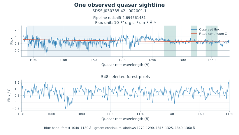
Transmission needs a denominator: the continuum flux the quasar would have supplied without this absorption. The observation does not directly measure that missing background. We fit a simple power law using three fixed quasar-rest-frame windows: 1270–1290, 1315–1325 and 1340–1360 angstroms. These redward windows anchor an extrapolation into the forest.

The windows retain 166 pixels. Inverse-variance weighting gives amplitude about 3.31429 at 1280 angstroms, in the original flux unit, and slope about −0.846066. An independent solver profiles out amplitude analytically at each slope, then performs a one-dimensional search. Its parameters agree with the two-dimensional least-squares solution to relative error below four parts in a billion.

That agreement checks the solution of the stated fitting problem. It does not establish the power law as the true unabsorbed continuum. The weighted residual sum is about 288.862 for nominally 164 degrees of freedom. Pixel correlations, emission structure and model mismatch are not fully included, so it is not converted into a certified goodness-of-fit probability.

In the figure, the continuum crosses the three redward fitting windows and extends into the forest. The assumed denominator is now visible alongside the measured flux.

\begin{aligned}C(\lambda)&=A\left(\frac{\lambda_{\rm rest}}{1280\,\mathrm{\mathring A}}\right)^p\\ F_i&=\frac{f_i}{C_i}\end{aligned}

f_i

is coadded pixel flux,

C_i

the fitted and extrapolated continuum, and

F_i

their ratio.

Fixed SDSS observed coadd, extrapolated continuum and unclipped forest ratios — SDSS J030335.42−002001.1: plate2068, MJD53386, fibre316. Blue shading marks the forest; green marks continuum windows. The continuum is our weighted power-law estimate. Lower-panel ratios retain noise below zero and above one. This is observed-derived data, distinct from the synthetic gas screen. Open the full figure

Reading: Fixed SDSS continuum and flux-statistics exercise

Keep the noisy ratios before averaging

The arithmetic mean over 548 retained pixels is 0.7461836. Sample variance is about 0.0996164. Temporarily treating the continuum as fixed and neglecting pixel correlations, the average diagonal noise variance divided by continuum squared is about 0.0355552. Subtraction gives about 0.0640612. This is a conditional noise correction, not a direct measurement of intrinsic cosmic gas variance.

There are 13 ratios below zero and 109 above one. Physical transmission lies between zero and one, but noisy flux, background subtraction and continuum estimation need not respect that interval. Clipping the observed ratios would change their mean, variance and distribution. The distribution uses 20 bins between −0.5 and 1.5, with one underflow and three overflow pixels reported separately.

Effective optical depth takes the negative logarithm after averaging, giving about 0.292784. Averaging individual negative logarithms is a different operation and is undefined over the real numbers for negative pixels.

The OR-zero mask gives mean 0.767696 and effective optical depth 0.264362. This difference records sensitivity to selection. Statistics belong to the particular pixels retained.

\begin{aligned}\overline F&=\frac1N\sum_{i=1}^{N}F_i\\\tau_{\rm eff}&=-\ln\overline F\end{aligned}

Average retained pixel ratios first. This effective optical depth requires a positive overall mean.

Reading: Fixed SDSS continuum and flux-statistics exercise

Move an assumption deliberately

Multiply the estimated continuum by 0.95 without changing observed flux. Mean transmission rises to about 0.785456 and effective optical depth falls to 0.241490. Multiplying by 1.05 gives mean 0.710651 and effective optical depth 0.341574. Raising the expected background makes the same received light appear more strongly absorbed.

Five percent is a chosen sensitivity perturbation, not a data-derived one-sigma uncertainty. Subtracting or adding 0.3 to the fitted slope gives means about 0.714569 and 0.779293. Amplitude and slope errors affect the extrapolated blueward continuum differently.

High signal-to-noise cannot replace checks of the object and continuum. If the mean ratio exceeds one, inspect emission structure, redshift and the continuum windows. A background estimate or target-identification problem may be exposed. Clipping the mean at one would hide that diagnostic.

Reading: Fixed SDSS continuum and flux-statistics exercise

Hand a reproducible result to the next physical question

Check file hash, units, redshift, windows, masks, continuum parameters and retained count before comparing the final statistics. The download supplies our calculation, input manifest and expected results. Running the script generates the derived pixel table. Fetch the original FITS separately from the named SDSS source. Reproduce the fixed example before substituting another object.

This result describes one sightline, one window and one continuum model. It does not include a complete instrument line-spread function, pixel covariance, metal rejection, damping-wing/BAL treatment or continuum covariance. Those omissions matter for gas temperatures and dark-matter inference.

The prescribed gas screen in the accompanying calculation sits at redshift three; these observed absorbers are at lower redshift. Similar mean fluxes would not constitute a fit. A physical inference must align simulated redshift, instrumental treatment, selection and statistical windows with the observations being explained.

Reading: SDSS DR17: Spectroscopic Data Basics · Fixed SDSS continuum and flux-statistics exercise

Exercises and explained answers

With observed flux fixed, what happens if the entire continuum rises by five percent?
Read the explanation
Every ratio is divided by 1.05, moving the mean from about 0.746184 to 0.710651. Effective optical depth increases by about 0.04879. This comes from the continuum assumption, not a newly observed change in gas density.
Why are forest absorber redshifts below the quasar redshift of about 2.69456?
Read the explanation
The light leaves the quasar and then crosses foreground gas. Quasar redshift locates rest-frame windows; each absorber is located by the observed wavelength of its pixel.

Try the prediction

Keep observed statistics separate from the forward model

Hold the numerical sightline fixed, record its mean transmission, and change only ionizing strength.
Explain how a specified incident continuum differs from the extrapolated continuum in an observation.
List what must be matched before fitting a redshift-three gas screen to this lower-redshift forest.

Independent calculations

Download the scientific ZIP · Read setup and scope

Python with NumPy and SciPy recalculates three synthetic spectra offline. The optional observed exercise also needs Astropy and the separately fetched, hash-pinned SDSS coadd. Instructions retain all pixels without clipping noisy ratios.

Scripts, file sizes and SHA-256

README.md (5881 B)
0f1259a35614944edbc800caab26c9ddfda8efcbdcadb76a1c407b6ee41c21db
calculate.py (1960 B)
789206ae0a4100c1ad25437d59c64f4b55d8482d9d4a03dfde040e900b727b2b
expected-observed.json (10116 B)
469a2191d51bf9050e1800df9ebb5e5b9aa3083da81db313f3cea8b5f2f28c12
expected-synthetic.json (51605 B)
1409ebb5261bcef0ab0871a40e48bdbce4a32404c08e9b6abe7a024ab7c56ade
fetch_sdss.py (1694 B)
23d8553b76c604c4e071411d845fe576f32471770313ae7e2e823c756c7ef32c
field-input.json (934 B)
1206529ed37acab5d72b1e83458c1db78f7a8cd579964ce01db4c02470c0dc43
input-manifest.json (651 B)
692fce6cd598d3bc14288384381afd24f7432d4e8f054fb94609e1a469e8dcdb
lyman-alpha-science-v1.zip (29960 B)
0a169f89a41770dd33b6bbefa7cda8ccd1d8579d0c77013ea77e0ccaa6112ea3
model.py (3656 B)
6a05678c4e50a5e4180aa8017633be68dcce3e7f16f55150df90edca9d465a22
sdss.py (6728 B)
4c9e99d73bfee1f07c9069caf1442f77cdee2cfba51fd079c06732759b6055be

Sources and calculation scope

Chen et al. (2017), published quasar target table: SDSS J030335.42−002001.1
Target-table entry used only to fix the published object name, position and approximate redshift 2.72 before flux analysis. The exact coadd instead supplies pipeline redshift 2.69456148147583. This was a targeted table reading, not a full-paper review.
SDSS DR17: Spectroscopic Data Basics
Official interpretation of calibrated coadds, vacuum heliocentric wavelengths, flux units, inverse variance, logarithmic sampling and AND/OR masks. The fixed file has 3,812 coadded pixels; it is not raw exposure data or a measured unabsorbed continuum.
Fixed SDSS continuum and flux-statistics exercise
Plate 2068/MJD 53386/fibre 316, run2d 26, SHA-256 83b81bfc16c91750030758d00646366ff2cada06b7f05a80ac97ad152fc387fa. Original FITS is fetched separately; derived ratios use stated continuum windows and masks. Noise correction is conditional on fixed continuum and diagonal noise, not a gas-temperature or cosmological inference.