Count atoms along a light path
Put the observer on the negative side and let light travel from the positive side. The comoving coordinate labels position on a grid that separates out the overall expansion. Begin with a short proper length . Neutral-hydrogen density counts neutral atoms per cubic centimetre.
A cross section , measured in square centimetres, describes one atom’s interaction with the selected light. This effective area depends on wavelength; it describes an interaction probability per incident photon. Density times cross section times path length has no units: it is that segment’s optical depth.
For uniform neutral density, density times length is the column density , in inverse square centimetres. As a counting example, take neutral atoms per cubic centimetre over two proper megaparsecs, about . The column is about . No velocity distribution has been specified yet.
Reading: Tepper García, Voigt profile fitting to quasar absorption lines, arXiv:astro-ph/0602124v1 · Independent hydrogen and sightline calculation materials
Find the part that still has electrons
The input gas density is usually total hydrogen . Its neutral fraction gives the neutral density when multiplied by the total. Assume pure hydrogen, a uniform radiation background and local ionization equilibrium. Each neutral atom is ionized at rate , while electrons and protons recombine with coefficient .
In pure hydrogen, electron and proton densities are equal: each is the total density times the ionized fraction. Substituting them into ionization balance gives the dimensionless expression below. measures recombination relative to photoionization.
When the neutral fraction is small, the ionized fraction is almost one and the neutral fraction is approximately . Doubling total density at fixed temperature and background then produces about four times as much neutral hydrogen, because both partners in a recombination become more abundant. Near neutrality, solve the complete equation instead of extending that square-law estimate.
The calculation uses the temperature-dependent total hydrogen recombination coefficient of Verner and Ferland. The radiation background is prescribed within this finite screen. Ionizing radiative transfer and self-shielding are not solved. The total case-A coefficient counts recombinations to all levels; reabsorption of their emitted photons is not followed.
Reading: Verner & Ferland, Atomic Data for Astrophysics: Radiative Recombination Rates, arXiv:astro-ph/9509083v1 · Independent hydrogen and sightline calculation materials
One population absorbs a range of velocities
Atoms move thermally even when their gas has no bulk motion. The thermal Doppler width grows as the square root of temperature. Here the proton mass approximates the hydrogen-atom mass. The velocity standard deviation is smaller than by a factor of square root two.
The excited state’s finite lifetime gives a natural width. Thermal velocities supply an approximately Gaussian distribution. Their convolution, a weighted sum over atomic velocities, gives a Voigt profile. Its natural wings do not abruptly vanish at a selected velocity.
Write the Voigt function as . The dimensionless offset is relative velocity divided by thermal width, and compares natural and thermal broadening. The area convention is . Dividing the integrated line strength by thermal width then gives the normalized cross section.
The atomic decay rate belongs to the excited state. The environmental rate in the preceding section ionizes neutral atoms. Increasing the radiation background changes how many absorbers remain; it does not change this transition’s lifetime.
Reading: Tepper García, Voigt profile fitting to quasar absorption lines, arXiv:astro-ph/0602124v1 · Independent hydrogen and sightline calculation materials
Convert the expanding grid to a proper path
Comoving coordinates follow the expanding grid, while the number density counts atoms per proper volume. The scale factor connects the two. Its subscript distinguishes it from the Voigt damping parameter.
At redshift three, the scale factor is one quarter. Eight comoving megaparsecs span two proper megaparsecs. Substituting the comoving length directly into the absorption integral would overcount the path by a factor of four.
Each location also needs its recession velocity . Expansion plus peculiar motion determines which spectral velocity its atoms absorb most strongly. The next chapter examines this mapping; for now, treat it as an input for every gas segment.
The integral sums positive spatial lengths. Light travels from positive toward negative position; that orders the cumulative dimming, while every absorption contribution stays positive.
Reading: Peeples et al., Pressure Support versus Thermal Broadening in the Lyman-alpha Forest, arXiv:0910.0256v3 · Independent hydrogen and sightline calculation materials
Add absorption before calculating the remaining light
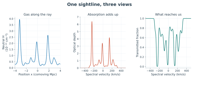
For every selected spectral velocity, traverse the same physical path. Each segment contributes optical depth. Add those depths and only then exponentiate to obtain transmission. Averaging the separate transmissions would describe parallel sightlines rather than successive segments.
If two segments have optical depths of 0.3 and 0.7 at one velocity, the total is one and about 36.8 percent of the background passes through. Reversing their order preserves this pure-attenuation result, although the positions at which the light dims are reversed.
A deep Lyman-alpha line does not require the screen to block all ionizing light. The line-centre cross section can greatly exceed the ionization-threshold continuum cross section. A small neutral abundance can therefore make a deep narrow line while the screen remains comparatively transparent to ionizing radiation. The declared ionizing-depth bound applies to this finite region.

Reading: Tepper García, Voigt profile fitting to quasar absorption lines, arXiv:astro-ph/0602124v1 · Independent hydrogen and sightline calculation materials
Finish with a limit you can integrate yourself
Take a uniform neutral density with no peculiar motion, expanding only with the Hubble flow. If the medium extends infinitely along the sightline, each spectral velocity encounters a complete copy of the same line profile. Changing the integration coordinate from proper distance to Hubble velocity leaves just the total cross-section area.
The resulting uniform Gunn–Peterson limit depends on neutral density, integrated line strength and Hubble rate. Here is the cosmic expansion rate in inverse seconds, distinct from the Voigt function .
A finite path omits the wings contributed by more distant gas. First compare it with an independent finite integral, then quantify the difference from the infinite-medium limit. Increasing the spatial quadrature resolution reduces discretization error; it does not restore gas excluded by the boundary.
Reading: Peeples et al., Pressure Support versus Thermal Broadening in the Lyman-alpha Forest, arXiv:0910.0256v3 · Independent hydrogen and sightline calculation materials