Why a Stretched Ripple Stops Changing After Horizon Exit

Two lengths to compare

Label points by comoving coordinates, which expand with space. A ripple then keeps a fixed comoving wavenumber $k$, while its physical wavelength $2\pi a/k$ grows with the scale factor $a$.

The Hubble length $1/H$ is the distance at which expansion carries two points apart at light speed. Points much closer than that can still exchange signals within one expansion time. Dividing by $a$ gives the comoving Hubble radius $1/(aH)$, the yardstick for a comoving ripple.

So the whole question is a comparison between $k$ and $aH$. A mode is inside the horizon when $k\gg aH$ and outside when $k\ll aH$.

Reading: Ellis, Vennin & Wands, Review 23: Inflation, Review of Particle Physics (PDG 2025, revised August 2025) · Adams, Cresswell & Easther, Inflationary perturbations from a potential with a step (2001), astro-ph/0102236v2

Inflation means a shrinking comoving Hubble radius

Because $aH=\dot a$, the comoving Hubble radius shrinks exactly when $\ddot a>0$. Accelerating expansion and a shrinking $1/(aH)$ are the same statement.

In e-fold time it is cleaner. With the Hubble slow-roll parameter $\epsilon=-\dot H/H^2$, the growth rate of $aH$ is $1-\epsilon$. Inflation is $\epsilon<1$, and we define its end as the moment $\epsilon=1$. On the Lab’s plateau, $\epsilon$ is only about $2\times10^{-4}$ when the pivot scale exits.

Reading: Ellis, Vennin & Wands, Review 23: Inflation, Review of Particle Physics (PDG 2025, revised August 2025) · Planck Collaboration, Planck 2018 results. X. Constraints on inflation, arXiv:1807.06211v2

Counting e-folds to horizon exit

A mode exits when $k=aH$. Two modes therefore exit $\int(1-\epsilon)\,dN=\ln(k_2/k_1)$ apart. When $\epsilon$ is tiny, the gap in e-folds is simply the logarithm of the wavenumber ratio.

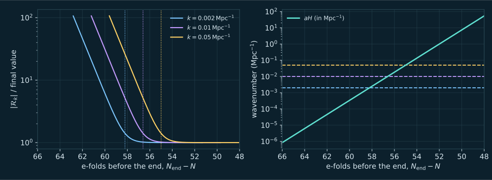
Worked example: the Lab tracks $0.002$, $0.01$ and $0.05\,\mathrm{Mpc}^{-1}$. The predicted gaps are $\ln 5\approx1.61$ and $\ln 25\approx3.22$ e-folds. In the computed figure the dotted exit lines sit near $58.2$, $56.6$ and $55.0$ e-folds before the end, which matches.

Those numbers need one convention to tie the model to real distances. We require that $k_*=0.05\,\mathrm{Mpc}^{-1}$ exits when $N_*$ e-folds of inflation remain. The default is $N_*=55$. Changing $N_*$ slides every observed scale along the potential.

Reading: Original background and mode calculations with an independent Python reference · Planck Collaboration, Planck 2018 results. X. Constraints on inflation, arXiv:1807.06211v2

Inside the horizon: a wave whose size falls

Deep inside the horizon, gravity barely matters on the scale of one wavelength. The field combination $v=z\mathcal{R}$ with $z=a\phi'$ then behaves like a free wave with fixed amplitude $1/\sqrt{2k}$.

Since $z$ grows almost like $a$, the curvature ripple $|\mathcal{R}_k|$ falls like $1/a$, by a factor $e$ per e-fold. The figure starts each mode at $k/aH=100$; over the next $4.6$ e-folds its size falls by about $100$, as $e^{4.6}\approx100$ predicts.

Reading: Adams, Cresswell & Easther, Inflationary perturbations from a potential with a step (2001), astro-ph/0102236v2 · Original background and mode calculations with an independent Python reference

Outside the horizon: why the ripple stays constant

The mode equation of the next chapter can be written in the conserved-flux form below. Once $k/aH\ll1$, the right-hand side vanishes, so $z^2aH\,\mathcal{R}'$ is constant.

Then $\mathcal{R}'\propto1/(z^2aH)$. With $z^2=2a^2\epsilon$ and slowly varying $H$ and $\epsilon$, this falls like $e^{-3N}$. One solution is constant; the other dies out within a few e-folds. That constant is the frozen value.

This conclusion relies on a single field. PDG 2025 notes that with several fields, non-adiabatic fluctuations can keep changing the curvature perturbation outside the horizon.

Reading: Ellis, Vennin & Wands, Review 23: Inflation, Review of Particle Physics (PDG 2025, revised August 2025) · Adams, Cresswell & Easther, Inflationary perturbations from a potential with a step (2001), astro-ph/0102236v2

What freezing does not mean

Freezing fixes each mode’s amplitude, not a predictable value. The frozen ripple is a random draw from the quantum state, so theory predicts its variance, the power spectrum $\mathcal{P}_{\mathcal{R}}(k)$. The Lab’s map is one such random draw.

After inflation, modes re-enter the growing horizon and start evolving again, becoming the acoustic patterns of the microwave background and the seeds of structure. Following that later evolution takes transfer functions, the next stage beyond this chapter’s model.

Reading: Ellis, Vennin & Wands, Review 23: Inflation, Review of Particle Physics (PDG 2025, revised August 2025) · Planck Collaboration, Planck 2018 results. X. Constraints on inflation, arXiv:1807.06211v2