What the Tilt, Tensors and Squeezed Triangles Measure

The tilt measures how fast the freezing conditions change

Define $n_s-1=d\ln\mathcal{P}_{\mathcal{R}}/d\ln k$. Each $k$ freezes when $k=aH$, and $d\ln k=(1-\epsilon)\,dN$ there, so the tilt measures how quickly $H^2/\epsilon$ changes per e-fold. To leading order in the potential slow-roll parameters this gives the expression below.

Worked example on the plateau at $\phi_*=5.3213$: $\epsilon_V=2.30\times10^{-4}$ and $\eta_V=V_{,\phi\phi}/V=-0.0173$, so $n_s\approx1-0.0360=0.9640$. The numerical spectrum, differenced between $0.049$ and $0.051\,\mathrm{Mpc}^{-1}$, gives $0.96490$. Leading order is good to about $10^{-3}$ here.

Reading: Ellis, Vennin & Wands, Review 23: Inflation, Review of Particle Physics (PDG 2025, revised August 2025) · Original background and mode calculations with an independent Python reference

Two potentials, two predictions

For the $R^2$ plateau, Planck 2018 X equation 48 quotes the lowest-order results $n_s-1\simeq-2/N$ and $r\simeq12/N^2$. At $N_*=55$ these give $0.9636$ and $0.00397$; the full calculation gives $0.9649$ and $0.00355$. The formulas are lowest order in $1/N$, and our $N$ counts to $\epsilon=1$.

For $\tfrac12m^2\phi^2$, $\epsilon_V=2/\phi^2$ and inflation ends near $\phi^2=2$, so $\phi_*^2\simeq4N+2$. Then $n_s-1\simeq-2/(N+\tfrac12)$ and $r\simeq8/(N+\tfrac12)$: $0.9640$ and $0.144$ at $N=55$. The numerical values are $0.9634$ and $0.1440$.

Both match Planck’s tilt. They differ by a factor of forty in $r$, which is what separates them.

Reading: Planck Collaboration, Planck 2018 results. X. Constraints on inflation, arXiv:1807.06211v2 · Original background and mode calculations with an independent Python reference

Tensors: the ratio that excludes the steep slope

Gravitational waves freeze like the curvature ripple but with friction $3-\epsilon$. At leading order $r=\mathcal{P}_t/\mathcal{P}_{\mathcal{R}}\simeq16\epsilon$, so $r$ measures the slope of the potential, and through $H$ the energy scale of inflation.

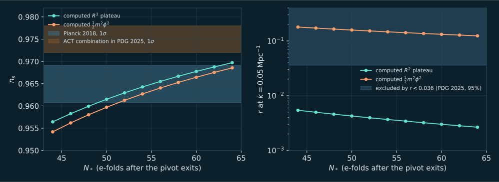
PDG 2025 quotes $r<0.036$ at $95\%$ confidence from BICEP, Keck Array and Planck data. The quadratic model gives $0.124$ to $0.179$ for $N_*$ between $64$ and $44$, three to five times too large, as the right-hand panel shows. The plateau sits well below the bound.

Always check the pivot. Planck 2018 X quotes $r_{0.002}<0.056$, at $k=0.002\,\mathrm{Mpc}^{-1}$. For the plateau our $r$ is $0.00318$ there and $0.00355$ at $0.05\,\mathrm{Mpc}^{-1}$. The Lab reports the value at $0.05\,\mathrm{Mpc}^{-1}$, because a large-scale step can distort $r_{0.002}$.

Reading: Ellis, Vennin & Wands, Review 23: Inflation, Review of Particle Physics (PDG 2025, revised August 2025) · Planck Collaboration, Planck 2018 results. X. Constraints on inflation, arXiv:1807.06211v2

Reheating moves the pivot along the potential

How many e-folds $N_*$ separate the pivot’s exit from the end of inflation depends on the expansion history afterwards, including reheating. PDG 2025 notes that the uncertainty in $n_s$ is comparable to the spread of many model predictions for $N_*$ between $50$ and $60$.

The left panel makes this concrete. On our grid the plateau runs from $n_s=0.9564$ at $N_*=44$ to $0.9697$ at $N_*=64$. It stays inside the Planck $1\sigma$ band for roughly $N_*$ from $49$ to $63$. The Lab’s shorter-reheating preset, $N_*=46$, gives $0.9583$.

So a tilt measurement constrains the potential and the post-inflation history together. That degeneracy returns in the reading guide.

Reading: Ellis, Vennin & Wands, Review 23: Inflation, Review of Particle Physics (PDG 2025, revised August 2025) · Original background and mode calculations with an independent Python reference

Squeezed triangles and the consistency relation

The three-point function $\langle\zeta\zeta\zeta\rangle$ depends on a triangle of wavenumbers. In the squeezed limit $k_1\ll k_2\simeq k_3$, the long mode froze long before the short ones. To them it is a constant rescaling of coordinates, which shifts their power by the tilt.

That gives the first relation below, the argument of Maldacena’s equation 1.2. Creminelli and Zaldarriaga showed it holds for any single-field model. With the sign convention used by Planck and PDG, which amounts to $\zeta=\zeta_g+\tfrac35f_{\mathrm{NL}}\zeta_g^2$, the local template has squeezed limit $\tfrac{12}{5}f_{\mathrm{NL}}P(k_1)P(k_2)$. Matching the two gives $f_{\mathrm{NL}}=5(1-n_s)/12$.

For $n_s=0.9649$ this is $0.0146$. Planck 2018 IX measured $f_{\mathrm{NL}}^{\mathrm{local}}=-0.9\pm5.1$, so the single-field value is about $350$ times smaller than the error bar. A clear detection of a local signal near $1$ would therefore point beyond a single field.

Reading: Maldacena, Non-Gaussian features of primordial fluctuations in single field inflationary models (2003), astro-ph/0210603v5 · Creminelli & Zaldarriaga, Single field consistency relation for the 3-point function (2004), astro-ph/0407059v2 · Ellis, Vennin & Wands, Review 23: Inflation, Review of Particle Physics (PDG 2025, revised August 2025) · Planck Collaboration, Planck 2018 results. IX. Constraints on primordial non-Gaussianity, arXiv:1905.05697v1

What the Lab’s squeezed readout is, and is not

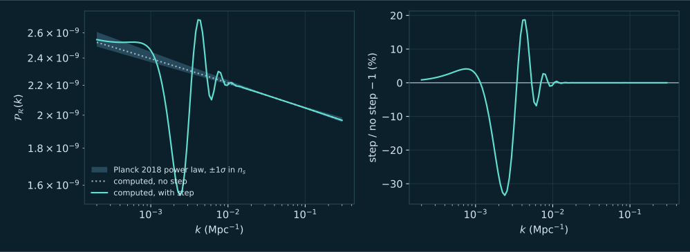
The Lab evaluates $\tfrac{5}{12}(1-n_s(k))$ with the local tilt of the computed spectrum at each short-mode $k$. On the smooth plateau it stays below $0.02$. With the default step the local tilt swings, and the largest value reaches $-0.651$; the exaggerated sharp step reaches $3.93$.

This is a restricted bispectrum: only the squeezed limit, and only through the consistency relation. Triangles with comparable sides need the full cubic interaction and are not computed. It covers only this limit of the step’s three-point signal. Even so, it shows that a feature in the spectrum must also appear in squeezed triangles.

Reading: Creminelli & Zaldarriaga, Single field consistency relation for the 3-point function (2004), astro-ph/0407059v2 · Original background and mode calculations with an independent Python reference