Today’s galaxies sit on a pattern that was laid down long before the first second ended. The leading explanation is inflation: a brief burst of accelerating expansion that stretched quantum jitters to enormous size and then froze them. Here is the path of one of those ripples.
Picture a ripple on a stretching sheet
Draw a small wave on a rubber sheet, then keep stretching the sheet faster and faster. Soon the wave’s crests are carried apart faster than anything on the sheet can travel from one crest to the next. That is roughly what inflation did to space.
The ripples themselves come from quantum physics. Even empty space holds a field whose value jitters slightly from place to place. During inflation one such field, the inflaton, also drives the expansion, so its jitters decide how long expansion lasts in each region.
Where inflation ran a little longer, space ended up stretched a little more. What survives is that difference in stretching, not the jitter itself. From here on, “ripple” means this difference.
A point on the sheet can only be influenced by points close enough for a signal to arrive within one expansion time. That distance is the horizon. During inflation the expansion rate barely changes, so the horizon keeps nearly the same size while every ripple is stretched far beyond it.
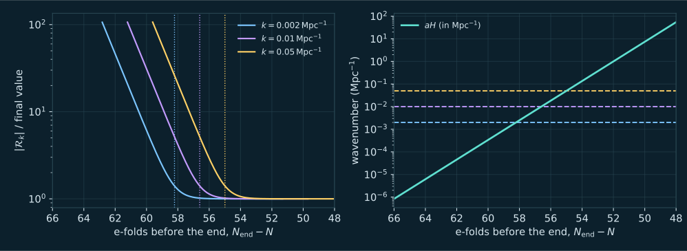
While a ripple is smaller than the horizon, it oscillates like a wave and its size keeps falling. Once it is stretched past the horizon, its two sides can no longer exchange signals, and its size stops changing. In the figure, three ripples of different length level off one after another.
The longest ripple freezes first. The shortest of the three, 25 times shorter, freezes about three e-folds later, where one e-fold means space has grown by a factor of about 2.7.
Our calculation for the smooth R2 plateau with N∗=55. Left or top: the size ∣Rk∣ of three complex mode functions, divided by its final value. Dotted lines mark k=aH. Right or bottom: aH in Mpc−1 rises while each fixed wavenumber stays flat; a mode exits where the lines cross. Model output, not data. Open the full figure
Because the expansion rate changes only slowly, ripples that freeze at different times come out with almost the same strength. The typical ripple Planck measured is about five parts in a hundred thousand.
The word almost matters. Planck 2018 found longer waves slightly stronger, a tilt measured as ns=0.9649±0.0042, where exactly 1 would mean equal strength at every size. That small departure records how the expansion rate eased off while the ripples froze.
PR(k)=As(k∗k)ns−1
The simple description Planck fits: strength As at a reference wavenumber k∗, with a tilt ns. A tilt below one gives longer waves, smaller k, slightly more power.
When inflation ended, its energy turned into hot matter and radiation. The frozen ripples became regions that were slightly denser or slightly emptier than average. Gravity then pulled matter towards the denser patches for billions of years.
Gravity strengthened the ripples and, on the largest scales, kept their statistics intact. The largest patterns in today’s universe therefore still carry information about that first instant.
In the simplest picture the inflaton rolls down a smooth hill of energy. If the hill had a small step, the field would lurch as it passed it. Ripples freezing at that moment would come out alternately stronger and weaker, a ringing pattern over a narrow range of sizes.
A lurch also makes the ripples less purely random: large and small ripples become linked. Cosmologists call this non-Gaussian. A smooth hill with one field predicts almost none, far below what current measurements can detect.
Planck looked for both. Its 2018 analysis found no preference for a step or for oscillating features, and its measurement of local non-Gaussianity was consistent with zero. The Lab lets you add an exaggerated step to see what such a signal would look like.
Inflation explains why the ripples are nearly equal in strength and why they tilt slightly. Other pieces are still missing. Gravitational waves from inflation have not been detected; the upper limit quoted by PDG 2025 already rules out the steepest simple hills.
Which ripples froze when depends on how the universe heated up after inflation, and that process is poorly known. The PDG 2025 review also reports a recent combination of ACT data with other measurements, which it calls not yet a full joint analysis. That combination prefers a slightly higher tilt, 0.975±0.003.
Two ripples differ in length by a factor of 25. Which one froze first, and roughly how much later did the other freeze?
Read the explanation
The longer one froze first, because the stretching carried it past the horizon sooner. Each e-fold multiplies lengths by about 2.7, and three e-folds give about 20, so the shorter ripple froze a little more than three e-folds later. The Lab’s tracked ripples at 0.002 and 0.05Mpc−1 show this gap.
Suppose Planck had measured a tilt of exactly 1. What would that have said about inflation?
Read the explanation
Ripples of every size would have the same strength, so the expansion rate would not have changed at all while they froze. The measured value just below 1 says the rate was slowly falling, which is what happens when the field rolls down a gentle hill.
Why does a small step on the hill change only a narrow range of ripple sizes?
Read the explanation
The field crosses the step quickly. Ripples that had already frozen keep their size, and ripples still far inside the horizon mostly settle back after the jolt. Only ripples near the horizon size at that moment are strongly changed, so the ringing sits around one band of sizes.
Open the Lab and let it play. The ball on the hill marks the time, and the dashed circle on the map shows the wavelength leaving the horizon at that moment.
Watch the mode-freezing chart below the stage. Each coloured curve falls and then flattens as its ripple exits the horizon.
Press Smooth plateau, then A step rings the spectrum, and compare the spectrum chart.
Full v2 PDF (2 August 2019) read for Sections 4.2 and 7.1–7.3: equations 47–48, the step template in equations 57–62, Table 11 priors, Table 12 step results and Figure 28. The headline spectral index and amplitude quoted in this course come from its parameter tables.
Full v1 PDF read for Sections 2.1–2.2 (equations 1–3, written for the Bardeen potential rather than the curvature perturbation), Table 5 final SMICA T+E values after lensing-ISW subtraction, and Table 10 feature-model peak statistics with the look-elsewhere correction.
Full review read. Used: Section 23.3.4 equations 23.55–23.57 and its sentence on the ACT combination, Section 23.6 on reheating and the number of e-folds after the pivot exits, and Section 23.7.3.2 equations 23.101–23.103 for the sign convention of the local non-Gaussian amplitude and its single-field squeezed-limit value.
Full v2 read. Equation 1 defines the tanh step we use; equations 6–19 set out the mode equation in e-fold time and its initial data. Our code is written independently and puts the step on the Starobinsky plateau and on a quadratic potential, not only on the paper’s quadratic case.
Our own calculations: the Lab integrator and a separate NumPy/SciPy reference agree to better than three parts in ten thousand on all five presets. The ZIP holds the Python reference, closed-form benchmarks, five inputs and expected outputs. No Engine code and no paper text is included.
Keep reading
What this page links to directly
You are hereHow a Quantum Ripple Becomes Cosmic Structure