Reading Planck’s Searches for Inflation Features and Non-Gaussianity
Sandbox Physics ·
This guide walks through the sections, tables and figures where Planck tested for features in the primordial spectrum and for non-Gaussianity, then through the PDG review that places those results beside newer data. For each claim it says who made it, in which version, and what kind of claim it is.
What to open, and what kind of source each one is
Planck 2018 X, Constraints on inflation, arXiv:1807.06211v2 dated 2 August 2019, and Planck 2018 IX, Constraints on primordial non-Gaussianity, arXiv:1905.05697v1. Both are collaboration papers prepared for Astronomy and Astrophysics; their numbers below are published measurements.
Review 23, Inflation, in the Review of Particle Physics, revised August 2025 by Ellis, Vennin and Wands. It is a published review that summarises newer results. Two of them are used here only as the review reports them: the ACT combination for the tilt, cited as arXiv:2503.14452, and the BICEP, Keck Array and Planck tensor bound. We did not read those papers.
Our own curves are model predictions from the Lab’s equations, checked by the independent Python reference. They are labelled as computed in every figure.
Section 7.1.2 models a tanh step in the potential, citing Adams, Cresswell and Easther, through a template written to second order. Equation 57 adds a first-order term I0 and a second-order term I1; equations 58–62 define them through window functions W0, W1 and a damping function D(x)=x/sinhx.
Three parameters set the feature: an amplitude As, a position ks and a damping width xs. Watch the notation. The symbol is the same one the paper uses elsewhere for the scalar amplitude, but here it means the size of the feature. Table 11 gives the priors: amplitude 0 to 1, log10(ks/Mpc−1) from −5 to −1 and lnxs from −1 to 5.
The Lab does not use this template. It integrates the mode equation for a tanh step directly. Its height, position and width map onto As, ks and xs only roughly, so we make no claim that a Lab preset reproduces a Planck fit.
lnPRs(k)=lnPR0(k)+I0(k)+ln[1+I12(k)]
Planck 2018 X equation 57, transcribed. PR0 is the featureless power law.
Sections 7.2–7.3 and Table 12: a better fit is not evidence
Section 7.2 fits each template to unbinned high-multipole likelihoods with nested sampling, holding nuisance parameters at their base-model best fit. Two numbers come out: the fit improvement Δχeff2 and the log Bayes factor lnB.
Table 12 gives the step model Δχeff2=−7.0 for temperature, −5.2 for E polarisation and −5.4 for the combination, with lnB=0.0, −0.2 and 0.1. Section 7.3 notes that these improvements fall within the range of about 10 expected from fitting noise. It adds that the best fit to the polarisation data is out of phase with the temperature fit, with log10ks=−3.47 against −3.11.
The conclusion in Section 7.3 is that the evidence for all models and data combinations lies between barely worth mentioning and substantial evidence against, so Planck shows no preference for these features. Three extra parameters will always buy some χ2; the Bayes factor charges for them.
Figure 28: a bound that applies to oscillations, not to steps
Figure 28 shows the modulation amplitude against frequency for the logarithmic and linear oscillation models of equation 56. Within the prior frequency ranges, the text states that the relative modulation is constrained to roughly 3%.
That bound concerns oscillations spread over all observed scales. A step makes a localised ripple at large scales, where cosmic variance is large, so the 3% figure does not carry over to the Lab’s step. Treat each bound as belonging to its own template.
Section 2.1 gives the equilateral and orthogonal templates, equations 1 and 2, for single-field models with non-standard dynamics. Section 2.2 gives the local template, equation 3, typical of several fields. All are written for the Bardeen potential Φ, not for ζ.
The final values come from Table 5, temperature plus E polarisation, lensing bias subtracted, KSW estimator: fNLlocal=−0.9±5.1, fNLequil=−26±47 and fNLortho=−38±24, at 68% confidence and statistical only. PDG 2025 rounds the local value to −1±5 in its equation 23.103.
Table 10 is the place to learn the look-elsewhere effect. For the feature bispectrum searches, raw peak significances of up to 3.0σ fall to at most 1.1σ once the size of the parameter survey is accounted for.
PDG 2025: the tilt, the tensor bound and reheating
Section 23.3.4 quotes Planck’s ns=0.9649±0.0042 in equation 23.55 and reports that ACT combined with Planck, lensing and DESI data suggests 0.975±0.003, adding that this is not yet a full joint analysis. Equation 23.57 gives r<0.036 at 95% confidence.
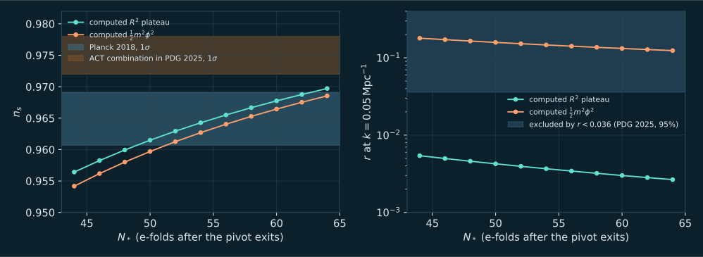
Section 23.6 explains why the tilt also tests reheating: within one model, ns and r depend on N∗, and the measurement error in ns is comparable to the change between N∗=50 and 60. Section 23.4.11 states that for the plateau-like class Planck allows 51<N∗<65. If the higher ACT value were confirmed, needing N∗>60 at 2σ, the simplest versions with conventional reheating would be ruled out.
Our computed curves show the same tension. The plateau stays inside Planck’s 1σ band for roughly N∗ from 49 to 63, and on our grid it reaches only 0.9697 at N∗=64, short of the ACT band. The small offsets from PDG’s range come from its lowest-order formulas and from where N is counted to.
Points are our numerical spectra for the R2 plateau and 21m2ϕ2, with ns from a finite difference at k=0.05Mpc−1. Bands are transcribed: Planck 2018 ns=0.9649±0.0042; the ACT combination 0.975±0.003, which PDG 2025 says is not yet a full joint analysis; and the PDG 2025 bound r<0.036 at 95% confidence. Open the full figure
Published measurements: Planck’s tilt, amplitude, feature fits and non-Gaussianity limits. Published review: the PDG summary and its reheating discussion. Reported but not read by us: the ACT combination and the tensor bound, both taken from the PDG text. Model predictions: equation 48 of Planck X and our numerical spectra.
Open questions: whether the higher tilt survives a full joint analysis; whether tensors will be detected; whether any large-scale feature is more than noise; how reheating fixes N∗; and whether squeezed non-Gaussianity well above the single-field value exists, which would point to more than one field.
Maldacena’s ns in equation 1.2 is the deviation from scale invariance, ns−1 in modern notation. Creminelli and Zaldarriaga’s equation 5 defines fNL with the opposite sign to Planck and PDG. Planck IX writes templates for Φ, which in the matter era equals 53ζ in Planck’s sign convention.
Planck X uses the symbol As for the scalar amplitude and, in Section 7.1.2, for the step amplitude. Tensor limits come at k=0.002 or 0.05Mpc−1. And N∗ depends on how the end of inflation is defined; we use ϵ=1.
The temperature step fit improves χ2 by 7.0 with three extra parameters, and lnB=0.0. Why is that not a detection?
Read the explanation
Section 7.3 says improvements of this size are within the roughly 10 expected from fitting noise. The Bayes factor of zero means the data do not prefer the step once its parameter volume is paid for. The polarisation fit lands at a different ks, out of phase with temperature, which a real feature would not do.
Planck’s temperature best fit has log10(ks/Mpc−1)=−3.11. With the Lab’s convention N∗=55, about how many e-folds before the end did that scale exit?
Read the explanation
ks=7.8×10⁻⁴Mpc−1, and ln(0.05/7.8×10−4)=4.17. It exited about 4.2 e-folds before the pivot, so about 59.2 e-folds before the end. This is close to the Lab’s default step, but the template amplitude does not map onto the step height, so it is not a fit.
Two papers report local fNL from the same data with opposite signs. What should you check first?
Read the explanation
The sign convention in the definition: ζ=ζg±53fNLζg2, or the equivalent for Φ. Creminelli and Zaldarriaga’s equation 5 uses the minus sign; Planck and PDG use the convention in which a positive value means a positive squeezed bispectrum of ζ.
A feature search reports a raw 3.0σ peak and a 1.1σ single-peak significance. Which do you quote?
Read the explanation
The corrected 1.1σ. The raw value ignores that many frequencies and phases were tried; the look-elsewhere correction accounts for the size of that survey.
Full v2 PDF (2 August 2019) read for Sections 4.2 and 7.1–7.3: equations 47–48, the step template in equations 57–62, Table 11 priors, Table 12 step results and Figure 28. The headline spectral index and amplitude quoted in this course come from its parameter tables.
Full v1 PDF read for Sections 2.1–2.2 (equations 1–3, written for the Bardeen potential rather than the curvature perturbation), Table 5 final SMICA T+E values after lensing-ISW subtraction, and Table 10 feature-model peak statistics with the look-elsewhere correction.
Full review read. Used: Section 23.3.4 equations 23.55–23.57 and its sentence on the ACT combination, Section 23.6 on reheating and the number of e-folds after the pivot exits, and Section 23.7.3.2 equations 23.101–23.103 for the sign convention of the local non-Gaussian amplitude and its single-field squeezed-limit value.
Full v2 read. Equation 1 defines the tanh step we use; equations 6–19 set out the mode equation in e-fold time and its initial data. Our code is written independently and puts the step on the Starobinsky plateau and on a quadratic potential, not only on the paper’s quadratic case.
Full v5 read. Equation 1.2 gives the squeezed-limit argument. In that paper the tilt symbol means the deviation from scale invariance, which modern papers write as the spectral index minus one.
Full v2 read. Equation 1 states the consistency relation for any single-field model. Equation 5 defines the local non-Gaussian amplitude with the opposite sign to Planck and PDG; we use the PDG sign and do not use or rewrite equation 6.
Our own calculations: the Lab integrator and a separate NumPy/SciPy reference agree to better than three parts in ten thousand on all five presets. The ZIP holds the Python reference, closed-form benchmarks, five inputs and expected outputs. No Engine code and no paper text is included.
Keep reading
What this page links to directly
You are hereReading Planck’s Searches for Inflation Features and Non-Gaussianity