Sandbox Physics
Galactic chemical evolution

Galactic chemical evolution · L3

From a gas track to a stellar abundance population

A curve through abundance space does not tell us how many stars occupy each part. A stellar population samples the gas composition at birth. Selection and measurement errors affect the population that we later observe. We will move from the gas record to a weighted birth population, then to a conditional measurement density. The distinction matters even when the gas evolution is numerically very accurate.

Weight births, not the length of the curve

For a constant return fraction, the mass locked into a stellar cohort during a short interval is proportional to the integral of the formation rate over that interval. A rapidly moving abundance track can contain very little stellar birth mass, while a slowly moving segment can contain much more. Normalizing these cohort masses gives the birth-mixture weights.

This is a population weighted by initial stellar birth mass, or equivalently by locked mass when the return fraction is constant. It is not yet a catalogue of present-day red giants. Red-giant lifetimes, luminosity cuts and membership selection require another weighting.

If abundance rises monotonically, changing variables from birth time to abundance introduces the inverse rate of abundance change. If a track loops, every birth-time branch must be included. A mixture over saved time intervals handles that without pretending that iron abundance is always a clock.

wj=ΔM⋆,j∑kΔM⋆,k,ΔM⋆,j=(1−R)∫tjtj+1ψ(t) dtw_j=\frac{\Delta M_{\star,j}}{\sum_k\Delta M_{\star,k}},\qquad \Delta M_{\star,j}=(1-R)\int_{t_j}^{t_{j+1}}\psi(t)\,dt
The weights are nonnegative and sum to one. The record saves the integrated mass and birth composition of each interval.
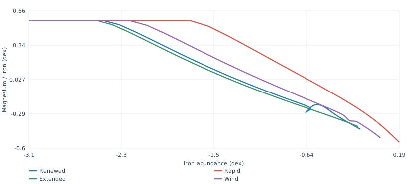
Four calculated gas abundance tracks, including a dilution loop
Original prescribed histories from saved gas inventories. These are gas tracks; curve length is not stellar birth mass. The renewed-supply track turns as new gas enters. No observed-star point is plotted. Open the full figure

Reading: Independent one-zone chemical-evolution Python materials

Average material before taking its logarithm

A birth group spanning an interval can have a changing gas composition. Average its element mass fractions with the formation-mass weights first, then convert those means into logarithmic abundances. Averaging already logarithmic values describes a different quantity.

For a worked example, let two portions have iron fractions 0.1 and 1 times the solar fraction, with birth masses in the ratio one to nine. Their mass-weighted fraction is 0.91 solar, whose bracket value is about minus 0.04096 dex. Averaging the two bracket values instead gives minus 0.1 dex. Neither arithmetic operation can be substituted for the other without changing the definition.

With the hydrogen fraction held at the same declared value as the solar conversion, the mass-fraction ratios map to the usual iron and magnesium-to-iron brackets. The atomic-mass factors cancel when the same element ratio is divided by its solar counterpart. Variable hydrogen enrichment would require a new conversion using the changing hydrogen fraction.

Reading: Independent one-zone chemical-evolution Python materials · VICE v1.3.1 fixed effective yields and solar reference

The iron measurement appears on both axes

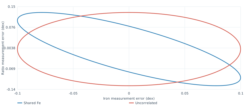
Write a measured iron error as eFee_{\rm Fe} and an independently measured absolute magnesium error as eMge_{\rm Mg}. The errors in iron abundance and magnesium-to-iron ratio are then eFee_{\rm Fe} and eMge_{\rm Mg} minus eFee_{\rm Fe}. The same iron error therefore enters them with opposite signs. Even independent absolute elemental errors generate a negative covariance in these plotted coordinates.

For independent errors of 0.10 dex in iron and 0.08 dex in absolute magnesium, the ratio error is about 0.12806 dex and the correlation coefficient is about minus 0.78087. The covariance matrix below follows from a linear coordinate transformation; it is not a measured covariance matrix for the Hill stars.

Σ=(0.0100−0.0100−0.01000.0164) dex2\Sigma=\begin{pmatrix}0.0100&-0.0100\\-0.0100&0.0164\end{pmatrix}\ \mathrm{dex}^2
The off-diagonal term is minus the iron variance. Dividing it by the product of the marginal standard deviations gives the correlation coefficient.
A negative shared-iron error ellipse and a zero-correlation ellipse with the same marginal errors
Original linear-error example, not the Hill covariance. Blue uses independent absolute iron and magnesium errors of 0.10 and 0.08 dex, transformed into iron and magnesium-to-iron coordinates. Orange keeps its marginal errors but sets correlation to zero. Curves are one-unit Gaussian quadratic contours, not calibrated confidence regions. Open the full figure

Reading: Independent one-zone chemical-evolution Python materials · Hill et al., VLT/FLAMES high-resolution chemical abundances in Sculptor, arXiv:1812.01486v2

Build a proper measurement density

Let each cohort mean be a point in the two abundance coordinates. For a measured star, place a normalized two-dimensional Gaussian around each cohort mean using that star's marginal measurement errors and an explicitly assumed correlation. The weighted sum is a mixture density. The determinant in the Gaussian normalization matters as much as the exponent.

A Gaussian is a bell-shaped cloud of measurement error around a modelled true value. A positive-definite covariance gives a positive variance in every direction. For marginal standard deviations σx\sigma_x and σy\sigma_y and correlation ρ\rho, this requires σx>0\sigma_x>0, σy>0\sigma_y>0 and ∣ρ∣<1|\rho|<1.

The determinant below controls the squared area scale of that cloud. Its square root has units of square dex and appears in the normalization; the inverse covariance weights deviations along the different directions of the error ellipse.

det⁡Σ=σx2σy2(1−ρ2)\det\Sigma=\sigma_x^2\sigma_y^2(1-\rho^2)
The correlation changes the area even when both marginal errors stay fixed. A normalized density must change its height accordingly.
p(a)=∑jwjexp⁡[−12(a−μj)TΣ−1(a−μj)]2πdet⁡Σp(\mathbf a)=\sum_j w_j\frac{\exp[-\tfrac12(\mathbf a-\boldsymbol\mu_j)^T\Sigma^{-1}(\mathbf a-\boldsymbol\mu_j)]}{2\pi\sqrt{\det\Sigma}}
Here a\mathbf a is the measured abundance pair, μj\boldsymbol\mu_j is a cohort mean and Σ\Sigma is the covariance for this measured star. The density integrates to one over the two-dimensional measurement plane.

Reading: Independent one-zone chemical-evolution Python materials

What a score can and cannot establish

The package reads saved measurements and saved cohort records to sum natural log densities. A density can exceed one because its units are inverse square dex; that is not a probability exceeding one. Correlations of minus 0.7, zero and plus 0.7 are separate sensitivity assumptions, not measurements of the unknown catalogue covariance. A model-axis offset of plus or minus 0.1 dex is likewise a scenario, not a calibrated solar correction.

The first attempted birth intervals of 0.02 and 0.01 gigayears gave a mean absolute change in per-star log density of about 0.08499, beyond the registered 0.01 gate. Accurate gas inventories did not rescue it. The finer 0.005 versus 0.0025 intervals pass the finite checks for four histories, both samples and the declared covariance and offset scenarios; a separate positive quadrature checks the observation integral.

For a real red-giant sample, unknown selection and shared abundance errors remain. The density is therefore a conditional teaching comparison, not a calibrated likelihood for a unique galaxy history. The held-out comparison uses these same conditional assumptions, including the unit birth-mass selection.

Reading: Independent one-zone chemical-evolution Python materials · Hill et al., VLT/FLAMES high-resolution chemical abundances in Sculptor, arXiv:1812.01486v2

Exercises and explained answers

  1. Two birth intervals have locked masses four and one. What are their normalized weights?

    Read the explanation

    Their weights are 0.8 and 0.2. The integrated stellar mass supplies the weight.

  2. If independent absolute iron and magnesium errors both have standard deviation 0.1 dex, what correlation appears between iron and magnesium-to-iron?

    Read the explanation

    The ratio variance is twice 0.01 square dex and the covariance is minus 0.01. The resulting correlation is minus one over the square root of two, about minus 0.7071.

  3. A prescribed history has the highest held-out density among four candidates. Is its star-formation history uniquely measured?

    Read the explanation

    No. The comparison is conditional on the yield model, solar conversion, covariance assumptions, birth weighting and the four offered candidates. Unknown red-giant selection and other histories remain outside it.

Try the prediction

Compare histories in one gas reservoir

  1. Choose a track segment where few stars form. Compare its geometric extent with the mass assigned to its birth groups.
  2. Export a cohort, calculate its logarithmic abundances from averaged birth fractions, and compare with an unweighted average of logarithms.

Sources and calculation scope

  1. Hill et al., VLT/FLAMES high-resolution chemical abundances in Sculptor, arXiv:1812.01486v2

    Main sections 1–7 and appendices A/B read again; Table C5 extracted in two text modes with exact agreement on 99 rows and 96 finite Mg/Fe pairs. Methods specify the 25-arcminute-diameter field and upper-RGB selection; conclusions use inconsistent radius wording. Full per-star covariance and a numerical model-solar harmonization are not established here. Original observations, PDF and measured-derived figures remain local.

  2. VICE v1.3.1 fixed effective yields and solar reference

    Previously frozen native defaults: Kroupa convention, effective net core-collapse and Type Ia magnesium/iron yields, Asplund 2009 reference and the declared hydrogen conversion. Public materials contain scalar values and identities, not a new yield grid or VICE executable. The independent Python does not execute VICE.

  3. Independent one-zone chemical-evolution Python materials

    Original continuous convolution/DOP853 producers, saved fourteen-field inventories and birth populations, finite refinement, normalized conditional mixtures and mathematical limits. Public inputs and figures are original synthetic data. Default is offline; optional fixed Hill source is fetched and analyzed on the reader’s computer. No App/Engine, original paper, observed rows or measured-derived plot is included.

FeedbackSomething broken, confusing, or missing on this page?Tell us
What kind of feedback?

Sent with this page’s address, its Lab ID, the site language and your device type. Please leave out personal details. Feedback is kept for up to 12 months.Privacy policy