A closed box gives an independent control
Start with no inflow, no wind and only a prompt net yield. Gas decreases as a fixed fraction of each new generation remains locked. Dividing the element-fraction rate by the gas-mass rate eliminates the formation rate. Integrating from the initial gas mass to the remaining gas gives:
Reading: Independent one-zone chemical-evolution Python materials · Weinberg, Andrews & Freudenburg, Equilibrium and Non-Equilibrium Aspects of Galactic Chemical Evolution, arXiv:1604.07435v1
Work through a half-depleted reservoir
With return fraction 0.4, prompt iron yield 0.000246 and initial iron fraction one millionth, half the initial gas remaining gives an iron fraction of approximately 0.000285190. The factor multiplying the natural logarithm is the yield divided by 0.6. The logarithm is , not .
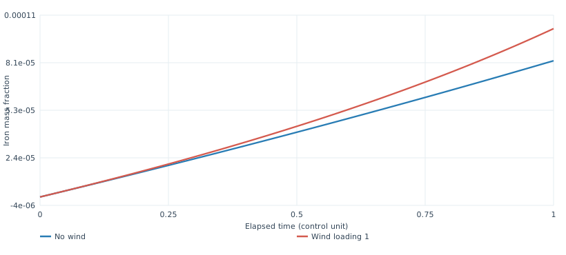
For a well-mixed wind, replace 0.6 in that factor by 0.6 plus . At the same remaining gas fraction, stronger loss means less new iron enrichment. At the same elapsed time under a prescribed formation history, however, it can leave less gas and a larger iron fraction. Our prompt-only control gives 0.00008236 without wind and 0.00010154 with one after the same time. Neither statement contradicts the other.
These controls isolate the prompt-only mathematical limit; the full calculation retains its original prompt and delayed effective yields.

Reading: Independent one-zone chemical-evolution Python materials · Weinberg, Andrews & Freudenburg, Equilibrium and Non-Equilibrium Aspects of Galactic Chemical Evolution, arXiv:1604.07435v1
Normalize a distribution of waiting times
A delay-time distribution tells us how a population releases its integrated delayed yield over time. In this package the dimensionless delay is the actual delay divided by one gigayear. The kernel is a power law between 0.15 and 15 gigayears and zero elsewhere. Its coefficient makes its integral over that entire interval equal to one.
Reading: Independent one-zone chemical-evolution Python materials · VICE v1.3.1 fixed effective yields and solar reference
Do not renormalize an unfinished history
Let be the integral of the kernel from its minimum delay up to a specified delay. At eight gigayears, is about 0.889076. Nearly eleven percent of the integrated delayed yield of an ideal population born at time zero still lies beyond that age. Stopping the simulation at eight gigayears does not make it legitimate to rescale the completed fraction to one.
For example, a million solar masses formed at once eventually contribute 2580 solar masses of new delayed iron under the fixed input. By eight gigayears they have delivered about 2293.82 solar masses. The small delayed magnesium yield similarly delivers about 7.85054 solar masses. These are cumulative new inputs before later locking or wind removal; they are not the gas inventories at eight gigayears.
Reading: Independent one-zone chemical-evolution Python materials · VICE v1.3.1 fixed effective yields and solar reference
Add all the earlier generations causally
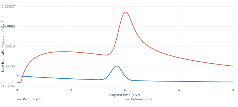
A generation born at time has delay when the clock reaches . Multiply its formation rate by the kernel at that delay, then add every eligible birth time. This is a causal convolution: no future star formation contributes to a present source.

Reading: Independent one-zone chemical-evolution Python materials · Weinberg, Andrews & Freudenburg, Equilibrium and Non-Equilibrium Aspects of Galactic Chemical Evolution, arXiv:1604.07435v1
Compute the source and the reservoir together
The independent Python calculation uses adaptive quadrature for the continuous convolution and a high-order differential-equation solver for the inventories. It integrates separately on each side of the first allowed delay, where the source switches on. Independent positive quadrature and a changed order of time integration check the source.
The reservoir starts slightly enriched: its iron fraction is one millionth, and its initial magnesium-to-iron ratio matches the fixed prompt yield ratio. No older stellar population is silently added to produce delayed events before the simulation begins. Inflow, the prescribed formation history and winds then act on the same gas record.
A knee in the stellar track depends on the competition among prompt sources, accumulated delayed sources, dilution and the times when stars actually form. It is not an exact marker of the first delayed event. The time integration, source quadrature and birth bins involve separate approximations. The reference checks the quantities affected by each of them.
After the gas trajectory is checked, the stellar population still requires accurate birth integration. The next chapter connects those weighted births to a measurement density, whose time integration receives a separate refinement test.
Reading: Independent one-zone chemical-evolution Python materials