Recompute a disk image and spectrum from saved intersections
Sandbox Physics ·
A disk image and its spectrum can be rebuilt from the same emitting points. Give each point a temperature and a frequency shift, then add its intensity with the area it occupies on the observer's sky. This guide follows one saved simulated intersection, one finite image cell and the complete fixed-aperture spectrum.
The downloadable tutorial supplies the two reference-rate states with inner edges at six and nine gravitational radii. Each has its own saved intersections and weights, three viewing directions and two integration levels. The calculation rebuilds local emission and weighted transport. Photon trajectories and the first opaque disk encounter remain frozen inputs. Read the first opaque encounter before changing what an intersection means.
Extract it and open a terminal in the extracted root, beside collection.json and source/. Python 3.12 or later is sufficient; the reader uses only the standard library. Run:
Both result.json files should report PASS_PORTABLE_EMISSION_AND_TRANSFER. Choose new output folders each time; existing records are preserved. These numerical inputs and Python code have been run in clean processes for both states, all three views at zero, sixty and seventy-five degrees, both levels and every one of the 257 original frequencies. The portable calculations passed their source comparisons and physical checks.
Both states use M=2×1031kg, inward rate M˙=1014kgs−1, distance D=1020m and colour hardening fcol=1.7. The emitting disk extends to six thousand gravitational radii. These are prescribed simulation inputs.
Keep geometry and expected answers apart
Open collection.json first. It names every array, shape, unit, column and source identity. For each state, input.npz contains endpoint geometry, first-hit status, original positive area weights, cell areas and the original frequency grid. The separate expected.npz contains reference radiometry and saved display arrays.
endpointIds gives view, ray, status and selected crossing order. endpointCoordinates gives the screen angle, path angle, emission radius and inverse-radius derivative. weightIds connects an endpoint to an integration level and a finite cell. A single endpoint can have more than one weight row. Follow those references instead of assuming that a row is a camera pixel.
A known nonhit emits zero. Its frequency ratio and effective temperature are not applicable, so the generated record marks them NaN and retains the original status. Undefined input coordinates keep their original NaN words. The surface-normal cosine remains reference-only. The emitter's arguments contain geometry. A separate controller compares each new return with its reference.
Follow endpoint 54626 from radius to intensity
Use the six-radius state at sixty degrees and fine level, index one. Endpoint 54626 is a HIT on ray 129. Its saved emission radius is r=12.0021, and its screen impact parameter is b=12.9414. Here distances in the formulas are numerical ratios to the gravitational radius rg=GM/c2, where G is Newton's constant and c is light speed. The two radii describe different places: one on the gas disk, one on the observer's screen.
Convert the emission radius to metres as R=r(GM/c2). With inner radius Rin, the prescribed one-face surface flux and effective temperature are
F(R)Teff=8πR33GMM˙(1−RRin),=(σSBF)1/4.
σSB is the Stefan–Boltzmann constant. This is the Newtonian zero-inner-torque law derived in Zimmerman et al., astro-ph/0408209v1, section 2. Where a thin disk heats follows that step from torque work. The downloaded code preserves the radius grouping above, including near the weak inner edge.
Next use the original screen angle χ=3.14866rad and inclination i, measured from the disk normal. In the supplied coordinate convention,
λg=−bcosχsini,=1−r−3/2λ1−3/r.
In SI terms, λ=Lzc/(E∞rg), with axial photon angular momentum Lz and energy at infinity E∞. The frequency ratio g compares arrival to emission. At this endpoint the new calculation returns Teff=1.95248×10⁶K and g=1.18562. The light is blueshifted along this direction; the local temperature still belongs to the gas.
For isotropic local emission, the arriving bolometric intensity is
Ibol,obs=πg4F.
It is 5.18308×10¹⁷Wm−2sr−1 here. For the monochromatic intensity, the two equivalent forms are
Bν is Planck's energy intensity per frequency. The code uses its SI form. The original three image channels are at 1016,1017,1018Hz. At the middle frequency this point gives 0.740035Wm−2sr−1Hz−1. Adding differently heated rings explains the thermal spectrum and colour hardening. Frequency and brightness shifts explains the cubic and fourth-power factors; Li et al., Appendix E gives the underlying intensity transport convention.
Add the original weights in cell 345
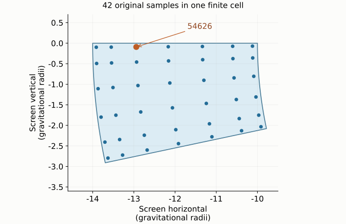
Weight row 59420 connects this endpoint to cell 345 at fine level. The cell lies on the observer's screen between impact parameters ten and fourteen, over one of thirty angular sectors. Its area is Ac=10.0531rg2. Its 42 original positive weight rows sample that finite region.
Original quadrature positions in screen cell 345, with endpoint 54626 highlighted. The cell is a finite image-plane sector, not a resolved camera pixel.
Let q index weight rows, e(q) their endpoint and k an image channel. The integrated cell intensity and its mean are
Jc,kIc,k=q→c∑wqIe(q),k,=AcJc,k.
The selected weight is 0.164410rg2, so its bolometric contribution is 8.52153×10¹⁶Wm−2sr−1rg2. Adding all 42 rows gives the cell integral 5.22431×10¹⁸Wm−2sr−1rg2. Dividing by the cell area gives mean intensity 5.19672×10¹⁷Wm−2sr−1.
Use the selected state's own cell area and radial panels. The six- and nine-radius grids have the same array shapes, but their physical boundaries differ. The mean intensity describes the whole finite cell.
Sum the same emission over the spectral aperture
At each of the 257 supplied frequencies, evaluate the same emitter and add every applicable original weight. Use the numerical area values in weightAreaRg2; one such area unit occupies (rg/D)2 steradians. The received flux is
Fν,obs=(Drg)2q∑wqIν,e(q).
The sum covers the original square extending 144 gravitational radii along each screen axis. The image-plane measure already supplies the viewing geometry; an additional flat cosine would change the calculation. The saved central image crop extends only 24 radii and leaves this sum unchanged.
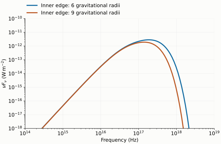
Actual recomputed reference-rate spectra at sixty degrees and fine level. The graph shows a frequency window; the supplied arrays retain the full original grid.
The fine bolometric lower flux is 5.58286×10⁻¹²Wm−2 for the six-radius state and 3.57953×10⁻¹²Wm−2 for the nine-radius state. These are simulated received fluxes through that finite aperture. The plot shows νFν over 1014 to 1019Hz; its logarithmic axes are a viewing choice. Frequency integration and all checks still use the original full grid.
The narrow unresolved critical band contributes a separately bounded unknown amount. The known-lower image and spectrum add the light from resolved directions. Retracing paths or making a new first-opacity decision requires a separate calculation and qualification. Here the prescribed Newtonian heating supplies emission at the frozen Schwarzschild intersections.
Read the checks and try the failure examples
The reader compares normal temperature, intensity and weighted outputs with the accepted same-source values at relative tolerance 10−12; frequency shift uses 10−10. These are arithmetic replay tolerances. Near a zero-torque inner edge, F64 agreement does not imply uniform accuracy for the continuum temperature. Zero/subnormal spectral tails instead use the original 1100-digit conditional positive-dot IEEE interval, conditional on the recomputed F64 intensities and original F64 weights. A ULP is the spacing between adjacent representable numbers; the audit reports absolute ULPs and unattainable relative precision. No independent Rin9 Decimal conditioning bound is claimed.
The separate physical checks retain the two-level spatial and spectral L1 limit of 10−3, unknown-light ratio 10−4, spectrum/bolometric agreement 10−8, 129/257-frequency consistency 10−3, and exact-area/solid-angle limit 10−12. Read a returned gate's actual value and limit together. A source, arithmetic or physical failure stops at its first error and keeps the returned prefix.
Why does a changed reference image leave the fresh image unchanged? The small fixture writes a bad expected image before starting a new calculation. The geometry-only emitter and original weights still generate the same actual image; the downstream comparison then rejects the reference. Damaging a real downloaded file also triggers its identity checks.
Can the nine-radius image be made by deleting six-radius endpoints inside nine? A path can pass through the larger inner hole and meet the disk later. The supplied nine-radius state therefore has its own first-hit table. An arbitrary new inner edge needs a newly qualified selection.
Should the two received fluxes have the exact inverse-inner-radius ratio? That scaling describes a particular Newtonian total-power comparison. A received finite-aperture flux also depends on which directions reach the disk and on their frequency shifts. Compare the actual sums above.
Which files let someone inspect your result? Keep result.json, the generated NPZ, both raw returned journals and the tail audits, together with the exact collection hash. They identify the data, calculation and first failure if one occurs. Full-precision teaching values are in the companion worked-example file; the numbers in the prose are rounded for reading.