How to read a thin-disk spectrum paper

By the end, you should be able to describe each panel's controlled comparison and explain why a harder spectrum alone cannot determine spin. Keep section 3.2, equations 14–17, Appendix E and section 4.2 beside the figure. The first pages explain model spectra; section 4.2 asks what additional information turns spectral fitting into a spin estimate.

Start with the quantity on each axis

Figure 5 plots observed photon energy horizontally and photon-number spectral flux density vertically. Both axes show base-ten logarithms. The energy unit is kiloelectronvolts; the vertical unit is photons per kiloelectronvolt, per square centimetre, per second. A horizontal coordinate of zero means one kiloelectronvolt. Moving one unit to the right multiplies energy by ten.

Let $E$ be photon energy and $N_E$ the photon-number spectral flux density. If energy is measured consistently in joules, $N_E$ counts photons per square metre, per second, per joule. The energy spectral flux density is

Every photon in the higher-energy bin carries more energy. To compare with a frequency spectrum, use $E=h\nu$, where $h$ is Planck's constant and $\nu$ is frequency. Matching the same small energy interval gives $F_\nu\,d\nu=F_E\,dE$, so

Multiplication by energy changes the curve's shape. A peak in photon number need not occur at the peak of energy per logarithmic frequency interval. Before comparing two plots, write the vertical quantity beside each one.

Try a conversion at one kiloelectronvolt. Suppose the photon spectrum there is one photon per kiloelectronvolt, per square centimetre, per second. One kiloelectronvolt is $1.602176634\times10^{-16}\,\mathrm{J}$, and one square centimetre is $10^{-4}\,\mathrm{m^2}$. The corresponding value is

The bin unit matters as much as the photon energy. The exact electronvolt conversion and Planck constant are listed in the NIST SI constants table.

Read the upper and lower panels separately

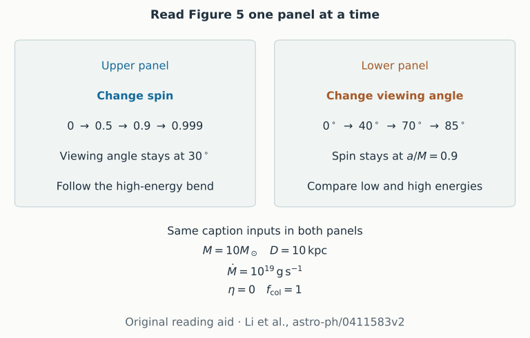
In the upper panel, the dimensionless spin $a/M$ takes the values $0,0.5,0.9,0.999$. The paper uses geometrized units for this ratio. The viewing angle stays at $30^\circ$, measured from the disk normal. All four curves use a mass of ten solar masses, a distance of ten kiloparsecs, an inward accretion rate of $10^{19}\,\mathrm{g\,s^{-1}}$, zero inner torque and colour hardening factor $f_{\rm col}=1$. The caption supplies these conditions. Section 3.2 also states that Figures 5–8 use isotropic emission in the gas frame.

The curves extend farther into the high-energy end as spin increases. Under the paper's assumption that the disk inner edge lies at the innermost stable circular orbit, a faster prograde spin permits emission closer to the centre. Those inner rings have higher temperatures. Section 3.2 also explains how radiation bent back onto the disk affects emission farther out. Follow both the emitting disk and the propagation when interpreting the change.

In the lower panel, spin stays at $a/M=0.9$. The viewing angles are $0^\circ,40^\circ,70^\circ,85^\circ$; the other caption parameters are unchanged. At low energy, the more inclined disk is dimmer. At high energy, the ordering changes. If inclination only multiplied every point by a projected-area cosine, the curves would keep the same order. Their crossing shows why the high-energy radiation requires the relativistic calculation. The paper attributes the enhancement to Doppler beaming and gravitational focusing.

“Harder” means that high-energy photons contribute more strongly relative to low-energy photons. It does not specify whether the change came from the local temperature, the viewing direction or another model assumption. Name the controlled change before using that word.

Follow Appendix E from the sky back to the gas

Equation E1 adds intensity over directions on the observer's sky. Here $F_E$ is received energy flux density, $I_E$ is intensity per solid angle and $d\Omega$ is an element of sky area measured in steradians. Equations E2–E3 introduce the frequency ratio $g$, observed photon energy divided by emitted photon energy:

The cubic factor and shifted energy argument belong together. Holding the emitted energy argument fixed would compare different photons. Equations E4–E6 then supply the effective temperature, the colour temperature and the diluted thermal intensity. Effective temperature describes the emitted total flux. Colour temperature shifts the thermal spectrum; its fourth-power dilution keeps the chosen total flux.

Read equation E7 as the combination of these steps. Different image directions can meet different disk temperatures and acquire different frequency shifts. Their intensities are added with the solid angle they occupy. This image-plane measure already describes how the disk appears to the observer; an extra flat projected-area factor cannot be appended to it.

For comparison, Zimmerman et al., astro-ph/0408209v1, section 2 derives a Newtonian thin disk with a zero-torque inner boundary. That is the local heating prescription used in this course's Schwarzschild examples. Li and colleagues use a relativistic Kerr disk and include returning radiation. The course examples keep the spacetime nonrotating and prescribe the inner edge; changing that edge supplies a heating-and-visibility comparison. Inferring spin requires a consistent Kerr emission and propagation model.

Continue to section 4.2 before claiming a spin estimate

Continuum fitting uses the smooth thermal part of a measured spectrum to estimate the disk's inner scale. Connecting that scale to spin requires an assumed relation between the inner edge and the innermost stable circular orbit. The mass $M$ sets the physical gravitational radius $GM/c^2$, where $G$ is Newton's constant and $c$ is the speed of light. The distance $D$ converts received flux into an intrinsic scale. The inclination $i$ changes projected area and the relativistic transfer. An independent estimate of each narrows the interpretations of the same spectrum.

Section 4.2 makes this dependence concrete. In the preceding normalization comparison, the authors varied distance while fixing spin. For their spin comparison, they use independent distances and vary spin and accretion rate. Read that change in fitted parameters before inspecting any quoted spin. The official XSPEC KERRBB manual lists mass, distance, inclination and spectral hardening as separate inputs, along with the inner-torque, self-irradiation and limb-darkening choices.

The atmosphere matters too. Absorption and scattering shape the light leaving the gas. A single colour hardening factor summarizes part of this physics, and section 4.2 discusses the resulting uncertainty. Figure 5 uses $f_{\rm col}=1$; the worked examples in this course use $1.7$. Two curves with different hardening assumptions cannot be treated as the same spin experiment. Instrument response, absorption along the line of sight and other spectral components also enter an observational fit; Figure 5 contains controlled model curves.

Read an iron-reflection spectrum alongside the thermal continuum

Thermal fitting follows the disk's own heat. Reflection follows X-rays from a hot corona that strike the disk and emerge after absorption, fluorescence and scattering. Iron fluorescence adds a line near $6\text{–}7\,\mathrm{keV}$, which orbital motion and gravity reshape. Its fit also needs the gas ionization and illumination model. The RELXILL authors' guide connects local reflection to relativistic propagation.

Open García and colleagues, arXiv:1312.3231v2, 12 December 2013, sections 1–4.1 and Fig.7 on PDF page 8. The left panel shows normalized energy spectra for four viewing inclinations. The middle panel divides the angle-dependent prediction by the usual angle-averaged convolution; those curves are model ratios, not observational residuals. The right panel shows how different local emission angles contribute to the received flux. Bending lets one observer receive photons emitted in several directions.

Try this check: would changing one overall normalization remove an energy-dependent middle-panel ratio? It would not. Record the angular treatment alongside inclination, ionization, iron abundance and illumination before interpreting a spin fit. Our thermal example supplies a comparison of emission and propagation; the reflection calculation belongs to the cited model.

Practise the reading on a new figure

A photon-number plot and an energy plot have different peaks. Which is wrong? Neither follows from that difference alone. Convert both to the same spectral quantity and units before comparing the peak locations.

Two inclination curves cross. Can one projected-area factor explain them? A constant factor changes every energy by the same proportion, so it cannot produce the crossing. Look for energy-dependent Doppler shifts and the image's gravitational distortion.

A hotter-looking spectrum gives a larger spin in a fit. What must you check? Start with which parameters were fixed, then examine their external measurements and uncertainties. Read the inner-edge, inner-stress and atmosphere assumptions with them.

Does a tighter image crop change the calculated full-aperture spectrum? A display-only crop leaves the integration unchanged. A smaller collection aperture discards light and can change the spectrum. Write down the actual aperture before comparing an image to a curve.

For the next paper, keep a short note with the source version and page, both axis quantities and units, the varied parameter, the fixed physical assumptions, the integration aperture and any external inputs used in fitting. That note tells you which comparison the figure actually supports.