Inferring a cooling age from brightness

Specify the clock and the hypothesis

A progenitor’s total age, a model’s elapsed white-dwarf cooling time and the independently reset time of a controlled thermal experiment are different coordinates. Subtracting one from another without matching their origins does not produce a physical age. Start by writing which clock you mean.

Let the hypothesis $H$ specify one native mass, progenitor composition, atmosphere and evolution calculation. On that fixed hypothesis, $t$ denotes elapsed cooling time in years. We do not interpolate mass or metallicity. A different atmosphere or mass is another hypothesis with its own conditional result.

A luminosity plateau makes the distinction especially important. Several times can have nearly the same luminosity, and a small measurement error may still allow a wide age range. Heating can also produce a local reversal. An age analysis therefore integrates over all supported times, including separate passages through the same brightness.

Sources: MIST white dwarf models, arXiv2509.21717v1, cooling clocks, surface boundary and model comparisons · Bédard, Blouin and Cheng 2024, Buoyant crystals halt the cooling of white dwarf stars, arXiv2409.04419v1, author manuscript of the Nature study, main text and Methods

Put the measurement and the model in the same coordinates

For Gaia-like photometry, use colour $c=G_{\rm BP}-G_{\rm RP}$ and absolute magnitude $M_G$ . With a high-significance parallax $\varpi$ in milliarcseconds, the inverse-parallax approximation gives the relation below. A model atmosphere maps native luminosity, effective temperature and surface gravity to those same two quantities.

The observational uncertainty must be stated in those coordinates. Independent mean-flux errors can be propagated to magnitude errors, and parallax uncertainty contributes to absolute magnitude. Calibration errors, extinction, atmospheric misclassification and unresolved binaries are additional issues; the reported formal errors do not automatically cover them.

Collect the two residuals in a vector $\mathbf d=\mathbf y_{\rm obs}-\mathbf y_H(t)$ . A covariance matrix $\Sigma$ contains the variances and their correlation. The quadratic residual below is dimensionless. In the teaching examples, we explicitly choose a diagonal covariance matrix. We do not add an adjustable scatter to hide a poor physical hypothesis.

M_G=G+5\log_{10}(\varpi_{\rm mas})-10,\qquad\chi^2(t)=\mathbf d^{\mathsf T}\Sigma^{-1}\mathbf d

The distance approximation is used only at high parallax signal-to-noise. Both components of the residual vector have magnitude units.

\mathcal L(\mathbf y_{\rm obs}\mid t,H)\propto\exp[-\chi^2(t)/2]

For a fixed, stated covariance this Gaussian likelihood compares predicted and observed photometry. It is not a model-discrepancy calibration.

Sources: MIST white dwarf models, arXiv2509.21717v1, cooling clocks, surface boundary and model comparisons · Bauer and Dotter, MIST white dwarf grid v1, Zenodo 15242047, CC BY 4.0 · Gaia DR3 archive data model, gaia_source fields

A prior over time is not a count of output rows

Bayes’ rule combines the likelihood with a prior $\pi(t\mid H)$ . Choose a proper uniform-time prior on a stated finite supported interval $[t_a,t_b]$ . Its density has inverse-year units. The posterior is then normalized by an integral over time.

A stellar code does not output equally spaced times. It takes smaller steps where the solution changes rapidly. Giving equal probability to every row would make the numerical solver’s step choices into an age prior. Refining a harmless part of the grid would then change the inferred age.

For an uninformative measurement and a uniform prior from zero to one gigayear, the median is half a gigayear. If a file happens to contain many rows near the beginning, that extra row count supplies no evidence that the star is young. Integration weights must represent elapsed time.

Even an evenly spaced logarithmic-age grid needs its Jacobian. Since $dt=(\ln10)t\,d\log_{10}t$ , equal logarithmic cells do not carry equal uniform-time prior mass. A uniform-log-age prior is another legitimate finite-interval choice, but it answers a different question and must be named.

p(t\mid\mathbf y,H)=\frac{\mathcal L(\mathbf y\mid t,H)\pi(t\mid H)}{\int_{t_a}^{t_b}\mathcal L(\mathbf y\mid t',H)\pi(t'\mid H)\,dt'},\qquad\pi(t\mid H)=\frac1{t_b-t_a}

The prior is zero outside the supported interval. This teaching prior specifies the time weighting under one model hypothesis; a Galactic star-formation history needs separate observational evidence.

Sources: MIST white dwarf models, arXiv2509.21717v1, cooling clocks, surface boundary and model comparisons · Bauer and Dotter, MIST white dwarf grid v1, Zenodo 15242047, CC BY 4.0

Work a synthetic example with a known answer

Define a hypothetical straight track for $0\leq t\leq1\,\mathrm{Gyr}$ : colour equals age in gigayears and absolute magnitude increases twice as fast. Observe colour $0.4$ and absolute magnitude $12.8$ , with independent assigned standard deviations $0.1$ and $0.2$ magnitudes. No noise is added; the ideal photometry corresponds to a known time.

Writing $u=t/(1\,\mathrm{Gyr})$ , the two residuals combine into a Gaussian centered at $u=0.4$ with standard deviation $0.1/\sqrt2$ . The proper prior truncates it to the supported interval. Its central sixteen-to-eighty-four-percent interval is about $[0.330,0.470]\,\mathrm{Gyr}$ , with median $0.400\,\mathrm{Gyr}$ .

These are posterior quantiles: they describe probability under the specified line, errors and prior. They are not a statement that this line is a physically correct white-dwarf model, or a demonstration of repeated-measurement coverage. A native-model holdout can test interpolation; independent stellar evidence is needed to test the physical hypothesis.

c_H(u)=u,\qquad M_{G,H}(u)=12+2u,\qquad\chi^2(u)=2\left(\frac{u-0.4}{0.1}\right)^2

This deliberately synthetic line is used by compute_textbook_examples.py. It contains no Gaia row or fitted catalogue age.

Sources: Bauer and Dotter, MIST white dwarf grid v1, Zenodo 15242047, CC BY 4.0 · Sandbox Physics, standalone white-dwarf scientific reference, original model inputs and independent tests

Integrate each time segment instead of trusting a few nodes

Between two neighbouring native times, interpolate the predicted two-component photometry linearly in fractional time $u\in[0,1]$ . Let $\Delta\mathbf y=\mathbf y_{i+1}-\mathbf y_i$ and $\mathbf d=\mathbf y_{\rm obs}-\mathbf y_i$ . Substitution into the likelihood makes the exponent a quadratic in $u$ .

Define the coefficients $a=\Delta\mathbf y^{\mathsf T}\Sigma^{-1}\Delta\mathbf y$ , $b=\mathbf d^{\mathsf T}\Sigma^{-1}\Delta\mathbf y$ and $c_0=\mathbf d^{\mathsf T}\Sigma^{-1}\mathbf d$ . Completing the square converts the time integral into a truncated-normal integral. Its prefactor includes the actual segment duration $\Delta t_i$ .

The formula below applies for $a>0$ . A completely flat joint-photometry segment needs a separate constant-likelihood treatment; the fixed-track reference rejects that unsupported extension. The supplied native tracks do not contain such segments. Stable log-CDF differences are used in the tails, and quantiles invert the cumulative probability within the selected segment.

The reference is checked against an independent adaptive numerical integral and against a rebinning of an identical straight track. Adding uneven output rows leaves both posterior and relative evidence unchanged. These checks test the numerical integration, not the stellar-evolution physics.

\chi^2(u)=a u^2-2bu+c_0,\qquad\mu=\frac ba

Here mu denotes the center in fractional time, not the mean particle mass from the envelope chapter.

\begin{aligned}I_i&=\int_{t_i}^{t_{i+1}}e^{-\chi^2(t)/2}\,dt\\&=\Delta t_i\sqrt{\frac{2\pi}{a}}\,e^{-(c_0-b^2/a)/2}\\&\quad\times\left[\Phi\!\left(\sqrt a(1-\mu)\right)-\Phi\!\left(-\sqrt a\,\mu\right)\right].\end{aligned}

Phi is the cumulative probability of a standard normal distribution. Summing these segment integrals and applying the declared prior gives the posterior normalization.

Sources: Bauer and Dotter, MIST white dwarf grid v1, Zenodo 15242047, CC BY 4.0 · Sandbox Physics, standalone white-dwarf scientific reference, original model inputs and independent tests

A normalized wrong answer is still wrong

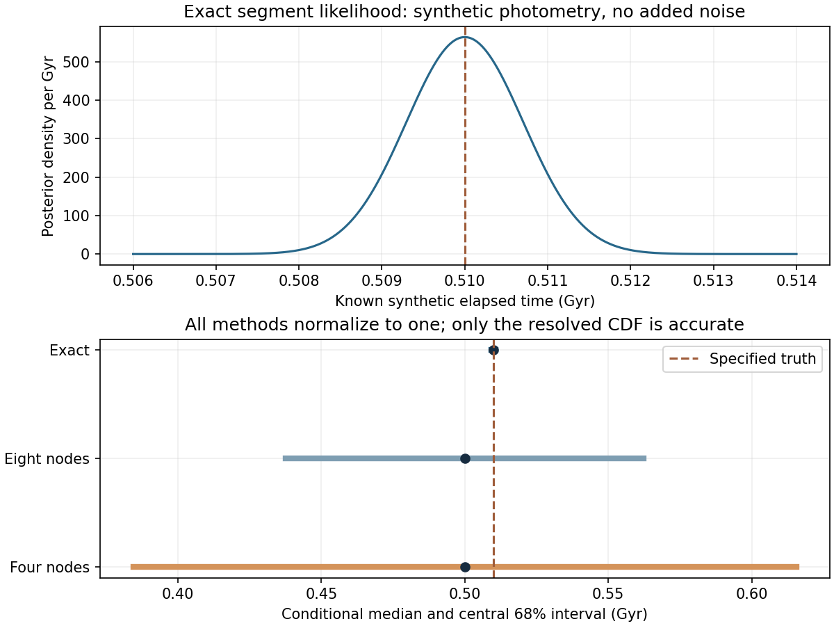
Keep the synthetic straight track but specify exact photometry at $0.510\,\mathrm{Gyr}$ with much smaller assigned errors: $0.001$ magnitude in colour and $0.002$ magnitude in absolute magnitude. The narrow likelihood lies between sparse quadrature nodes.

A retained failed method treats four or eight Gauss nodes as a discrete approximation to posterior probability and interpolates their accumulated weights. Both versions report a probability sum of one. Both put the median at half a gigayear, well away from the known value, and return grossly overwide intervals. The continuous model itself has a perfect photometric match; searching only the nodes even misses that match.

Exact segment integration recovers the known center and the narrow interval. The failure is computational, so the remedy is a better integral and CDF. Adding invented model noise would change the scientific question instead of fixing the integration.

After the numerical method passes, a real candidate can still fit a native mass or atmosphere hypothesis poorly. Keep that failure visible. Different model families retain independent clock origins, and their conditional age distributions should be compared without relabelling one as a calibrated age for the whole observed population.

Method	Median	Central68% interval
Four nodes	$0.500\,\mathrm{Gyr}$	$[0.384,0.616]\,\mathrm{Gyr}$
Eight nodes	$0.500\,\mathrm{Gyr}$	$[0.438,0.562]\,\mathrm{Gyr}$
Exact segment integral	$0.510\,\mathrm{Gyr}$	$[0.509297,0.510703]\,\mathrm{Gyr}$

Exact synthetic age likelihood and the incorrect four-node and eight-node intervals — Known synthetic time of 510 million years, with explicitly assigned photometric errors and no added noise. The exact likelihood is narrow; sparse-node CDF approximations normalize to one but return displaced medians and greatly inflated intervals. All quantities are recomputed from the hypothetical straight track.

Sources: Sandbox Physics, standalone white-dwarf scientific reference, original model inputs and independent tests · Bédard, Blouin and Cheng 2024, Buoyant crystals halt the cooling of white dwarf stars, arXiv2409.04419v1, author manuscript of the Nature study, main text and Methods