A tug together can become a drift apart
Picture stars moving around the Galaxy in a narrow band. A massive object passes nearby and pulls stars on both sides toward the encounter. At first those stars converge. Counting them in a short segment can show an enhancement.
Their subsequent motion is not straight-line travel. A small forward kick can put a star on an orbit with a larger mean radius. In a host with nearly constant circular speed, the larger circuit takes longer. That star initially moves forward, yet eventually falls behind. A backward kick can reduce the guiding radius and shorten the orbital clock.
The useful question is therefore not simply which star is faster now. Ask which orbit it occupies and how long each circuit takes. Small differences in those clocks accumulate until stars move away from the original encounter region.
Reading: Erkal & Belokurov (2015), Forensics of Subhalo-Stream Encounters, arXiv:1412.6035v2 · Sandbox Physics standalone stellar-stream scientific reader v1
One thin stream contains many orbits
The Galaxy pulls differently on the near and far sides of a cluster or dwarf galaxy. Those tidal differences can gradually remove stars and produce a stream. Escaping stars have slightly different positions and velocities. They spread along their orbits into a long band rather than following one identical path.
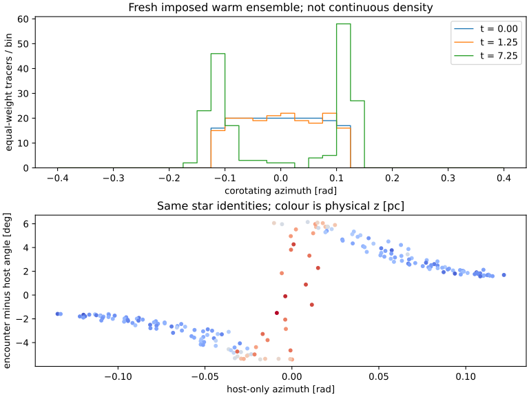
Our experiment starts later in that story, with an imposed warm segment of 192 tracers. Warm means a small initial spread of positions and velocities. Every tracer follows its own three-dimensional trajectory, but the calculation does not release stars from a progenitor or include their mutual gravity. It asks what a passing force does to an existing ensemble.
Reading: Erkal & Belokurov (2015), Forensics of Subhalo-Stream Encounters, arXiv:1412.6035v2 · Sandbox Physics standalone stellar-stream scientific reader v1
Put a number on the long memory
Two nearly circular orbital periods differing by one percent accumulate a phase difference of about a tenth of a turn, roughly thirty-six degrees, over ten circuits. Small clock differences become appreciable position differences. The time for an actual gap to develop also depends on how the kick varies along the stream.
For a more familiar scale, a velocity difference of one kilometre per second sustained for a hundred million years corresponds to about 102 parsecs of free straight-line travel. Galactic gravity bends the actual motion, so this is not a gap-width formula. It does explain why a modest disturbance can leave an extended trace.
Reading: Erkal & Belokurov (2015), Forensics of Subhalo-Stream Encounters, arXiv:1412.6035v2 · Sandbox Physics standalone stellar-stream scientific reader v1
Does the gap identify dark matter?
A small clump of dark matter bound within the Galaxy, called a dark subhalo, can perturb a stream without producing an obvious patch of light. That makes streams attractive probes of unseen mass. Ordinary massive objects also exert gravity, however, and variations in stellar release, smooth-potential orbital pile-ups and observational selection can change a count profile.
Position offsets, velocities, distances and chemistry add information. They need to be compared through the same observational selection. A striking gap, or an attractive fitted orbit, is not a unique verdict about the perturber. The thin stream and broad cocoon of GD-1 make that distinction particularly interesting.
Reading: Erkal & Belokurov (2015), Forensics of Subhalo-Stream Encounters, arXiv:1412.6035v2 · Valluri et al. (2025), GD-1 Stellar Stream and Cocoon in the DESI Early Data Release, arXiv:2407.06336v2
Make a prediction before changing the scene
Compare the compact and diffuse encounters at the same saved time. They use the same mass but distribute it differently; a more extended object produces a weaker nearby force gradient. Look at the saved counts and displacement diagnostics as well as the stars.
Then inspect the unperturbed reference. Losing a single tracer from a bin containing only a few stars can make a large ratio change. Counts outside the plotted range and the valid-ratio mask matter. These finite samples are not a continuous luminosity map.
Reading: Erkal & Belokurov (2015), Forensics of Subhalo-Stream Encounters, arXiv:1412.6035v2 · Sandbox Physics standalone stellar-stream scientific reader v1