Sandbox Physics
From ripples to the cosmic web

From ripples to the cosmic web · L2

Why One Position Can Have Several Velocities

After shell crossing, several material labels can reach the same position with different velocities. A location no longer identifies a unique origin. Its density adds the positive mass contributions of every stream.

A map that follows the matter

Compress matter along one direction and leave the other two uniform. The coordinate qq labels its uniform reference position; y(q,a)y(q,a) is its later comoving position. At the actual start, a particle is already at q+ais(q)q+a_i s(q). The unperturbed label and the displaced initial position are different arrays.

In the matter-only background the Zel’dovich growth factor is aa. Choose a sinusoidal displacement with amplitude AA, placing the strongest compression at the box centre. The plus sign below includes this phase choice.

y(q,a)=q+aA2πsin⁡(2πq),0≤q<1y(q,a)=q+\frac{aA}{2\pi}\sin(2\pi q),\qquad 0\leq q<1
Both coordinates are in box-length units. Each label keeps the same mass. Only the one direction of planar motion is changing here.

Reading: Zel’dovich (1970), Gravitational instability: an approximate theory for large density perturbations · Original finite-mesh calculations and independent small-wave Python replay

Measure how much an interval shrinks

Neighbouring layers separated by dqdq later span approximately dy=J dqdy=J\,dq, where J=∂y/∂qJ=\partial y/\partial q. This local stretching factor is a Jacobian. In three dimensions it becomes a determinant describing a volume ratio.

Before crossing, JJ is positive everywhere. Compressing the same reference mass into one-quarter of its former length gives four times the mean density. Transverse stretching is unchanged in this planar example, leaving just this length factor.

J=1+aAcos⁡(2πq),ρρˉ=1Jbefore crossingJ=1+aA\cos(2\pi q),\qquad\frac{\rho}{\bar\rho}=\frac1J\quad\text{before crossing}
The mean density already includes the background expansion. The ratio measures extra compression relative to the average at the same epoch.

Reading: Zel’dovich (1970), Gravitational instability: an approximate theory for large density perturbations

Calculate the first fold

Set A=1.8A=1.8. At the central label q=0.5q=0.5, the cosine is minus one, so J=1−aAJ=1-aA. At a=0.4a=0.4, this gives J=1−0.4×1.8=0.28J=1-0.4\times1.8=0.28 and a displacement-reference density about 3.573.57 times the mean.

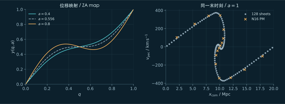
The first zero occurs at ac=1/A=5/9≃0.556a_c=1/A=5/9\simeq0.556. The map first becomes flat there, then develops a backwards-folding interval. The left panel follows this reference map. The other panel separately examines particle velocities after crossing.

A continuous, initially cold model develops a density singularity where J=0J=0. The local volume ratio approaches zero, without adding mass. A finite initial velocity spread or averaging over a finite volume broadens the peak.

ρρˉ∣q=1/2,a=0.4=11−1.8×0.4=10.28≃3.57\left.\frac{\rho}{\bar\rho}\right|_{q=1/2,a=0.4}=\frac1{1-1.8\times0.4}=\frac1{0.28}\simeq3.57
This is an analytic pre-crossing displacement value. A finite mesh peak also depends on mass assignment and force resolution.
Analytic plane displacement folds and the independent sheet versus PM phase-space comparison
Left/top: the analytic ZA map for A=1.8A=1.8 at three labelled epochs. Right/bottom: actual accepted phase-two PM and independent periodic sheets at a=1a=1, with peculiar velocity in km/s. PM has 1616 particles and mesh nodes per axis with a finite force cutoff; the reference has 128128 infinitesimal plane sheets. Their differing force resolution and sampling remain visible. Open the full figure

Reading: Zel’dovich (1970), Gravitational instability: an approximate theory for large density perturbations · Original finite-mesh calculations and independent small-wave Python replay

Tracing a position backwards gives three answers

Continue the same reference to a=0.8a=0.8. A horizontal line through the central position can intersect the folded curve three times. One yy now has three qq values. A label still gives a definite position, but the inverse lookup is no longer unique.

Those layers also have different velocities. Matter starting on the left can move right, a layer from the right can move left, and symmetry keeps the middle layer at the centre. Position superposes them; a position–velocity plot separates the streams.

The middle interval has negative JJ, marking a reversed ordering of labels. It has no negative mass. Find every branch at a location and add contributions using the absolute size of each local volume.

ρ(y)ρˉ=∑qs: y(qs)=y1∣J(qs)∣\frac{\rho(y)}{\bar\rho}=\sum_{q_s:\,y(q_s)=y}\frac1{|J(q_s)|}
The sum covers all streams at the location, with equal mass per uniform reference interval. A signed inverse Jacobian would confuse orientation with mass.

Reading: Zel’dovich (1970), Gravitational instability: an approximate theory for large density perturbations · Original finite-mesh calculations and independent small-wave Python replay

Let gravity respond after the fold

An extended displacement map still illustrates overlapping streams. Following their later motion requires gravity to respond to the new density. The streams continue attracting one another and changing velocity. Our independent periodic sheet reference calculates force from sorted mass; the mesh model distributes mass among finite nodes.

The post-crossing comparison uses a=1a=1 and the same sinusoidal initial condition for a three-dimensional PM plane with 1616 cells per axis and an unsoftened 128128-sheet reference. Match their cumulative mass from left to right and average the position differences to obtain the mass-quantile distance. Refining both particles and mesh to 3232 per axis reduces it from about 0.0176L0.0176L to 0.00860L0.00860L. This changes mass sampling and force resolution together.

One position can no longer carry a single velocity. Particle labels and positive mass let us follow several streams onward. The next chapter examines how a finite mesh turns those positions into a gravitational force.

Reading: Springel (2005), The cosmological simulation code GADGET-2, astro-ph/0505010v1 · Original finite-mesh calculations and independent small-wave Python replay

Exercises and explained answers

  1. How does the reference first-crossing scale factor change if A=1.8A=1.8 becomes A=0.9A=0.9?

    Read the explanation

    Because ac=1/Aa_c=1/A, it doubles from 5/95/9 to 10/910/9. A smaller initial ripple needs a larger growth factor to reach its first fold.

  2. After crossing, a branch has J=−0.4J=-0.4. What density does it contribute?

    Read the explanation

    It contributes 1/∣J∣=2.51/|J|=2.5 times the mean for uniform reference labels. Other branches add their own positive contributions. The sign only records orientation.

  3. If the first-crossing map locally has y−yc∝(q−qc)3y-y_c\propto(q-q_c)^3, how does density scale with distance from its centre?

    Read the explanation

    Differentiation gives J∝(q−qc)2J\propto(q-q_c)^2. Since ∣q−qc∣∝∣y−yc∣1/3|q-q_c|\propto|y-y_c|^{1/3}, inversion yields ρ∝∣y−yc∣−2/3\rho\propto|y-y_c|^{-2/3}. This follows from the specified local cubic model; it is not the exponent of every later fold.

Try the prediction

Separate overlapping positions with velocity

  1. Choose A sheet folds. Predict the first displacement-reference fold near a=0.556a=0.556, then inspect the actual ordering of the PM gold line and note whether they occur in the same native frame.
  2. Move beyond crossing and look for points with similar positions but different velocities in the external phase-space plot.
  3. Rotate the box to identify the plane, then compare the displacement reference. Explain how stream crossing differs from crossing a periodic face.

Sources and calculation scope

  1. Zel’dovich (1970), Gravitational instability: an approximate theory for large density perturbations

    All six original pages read. Physical displacement in the original notation is distinguished from modern comoving growth and canonical momentum. We use the pre-crossing map; its discussion of gas shocks is not applied to collisionless matter. The hosted paper remains external.

  2. Springel (2005), The cosmological simulation code GADGET-2, astro-ph/0505010v1

    Focused reading: Section 2.1, equations 1–3; Section 3.2/3.2.1, equations 20–23; Section 4.1, equations 26–31, with original pages 3 and 11 viewed. Supplies cosmological momentum, PM windows and time-integration context. The teaching calculation specifies its own cutoff and finite gradient and adds no short-range tree force.

  3. Original finite-mesh calculations and independent small-wave Python replay

    Original accepted kernel/linear, nonlinear and five-preset F64 calculations support the teaching figures and calibration. This small public ZIP contains only an exact current-state small-wave fixture, an independent NumPy/SciPy trajectory replay and expected output. The fixture was generated through the frozen model and canonical serializer in Node, not downloaded in a browser. Large raw preset archives remain separately retained; no Engine or source paper is included.

FeedbackSomething broken, confusing, or missing on this page?Tell us
What kind of feedback?

Sent with this page’s address, its Lab ID, the site language and your device type. Please leave out personal details. Feedback is kept for up to 12 months.Privacy policy