Sandbox Physics
From ripples to the cosmic web

From ripples to the cosmic web · L3

What a Power Spectrum Remembers

Power records the strength of fluctuations at a scale while discarding how the waves line up. It can test growth and still assign identical numbers to different spatial patterns.

Give each particle a direction on a circle

To look for the longest wave along a box axis, map each particle’s comoving position to one turn around a unit circle. Average the resulting arrows. Uniform coverage cancels their directions; a preference for some parts of the wave leaves an arrow with both length and direction. Its length measures amplitude and its direction records phase.

For a three-dimensional integer wavevector n\boldsymbol n, the complex exponential below stores both components. All masses are equal here, so all particles carry equal weight. We use nonzero modes; the mean density belongs to the background.

δn=1Np∑p=1Npexp⁡(−2πin⋅yp),n≠0\delta_{\boldsymbol n}=\frac{1}{N_p}\sum_{p=1}^{N_p}\exp(-2\pi i\boldsymbol n\cdot\boldsymbol y_p),\qquad \boldsymbol n\ne\boldsymbol0
The real part averages cosine and the imaginary part averages minus sine. Moving across a periodic face changes the phase by a whole turn and leaves this amplitude unchanged.

Reading: Original finite-mesh calculations and independent small-wave Python replay · Springel et al., First results from IllustrisTNG: matter and galaxy clustering (2018), arXiv:1707.03397v2

Squaring removes the direction

Square the arrow’s length and multiply by the comoving box volume. That defines power for a single discrete mode in this course. It has volume units: using Mpc for the box length gives Mpc3\mathrm{Mpc}^3. We do not multiply by the changing physical volume as the universe expands.

A usual cosmological power spectrum also averages modes with nearby wavenumber lengths and different directions, or describes an ensemble expectation. The Lab tracks a few specified modes. A single low-mode readout is not a precision measurement of an entire isotropic spectrum.

Pn=L3∣δn∣2,kn=2π∣n∣LP_{\boldsymbol n}=L^3|\delta_{\boldsymbol n}|^2,\qquad k_{\boldsymbol n}=\frac{2\pi|\boldsymbol n|}{L}
Before comparing a paper, check its volume normalisation, length units and mode averaging.

Reading: Original finite-mesh calculations and independent small-wave Python replay · Springel et al., First results from IllustrisTNG: matter and galaxy clustering (2018), arXiv:1707.03397v2

The same powers can draw different patterns

Superpose two small waves in one periodic coordinate: one goes around the box once and the other twice. Reverse the sign of the second wave. This shifts its phase by half a turn without changing either wave’s amplitude, while changing how their peaks meet.

The figure is our own continuous-density example, not PM output. Both densities stay positive. Both modes have power 20 Mpc320\,\mathrm{Mpc}^3 in each example, yet the spatial patterns differ. Those powers alone cannot uniquely reconstruct the image.

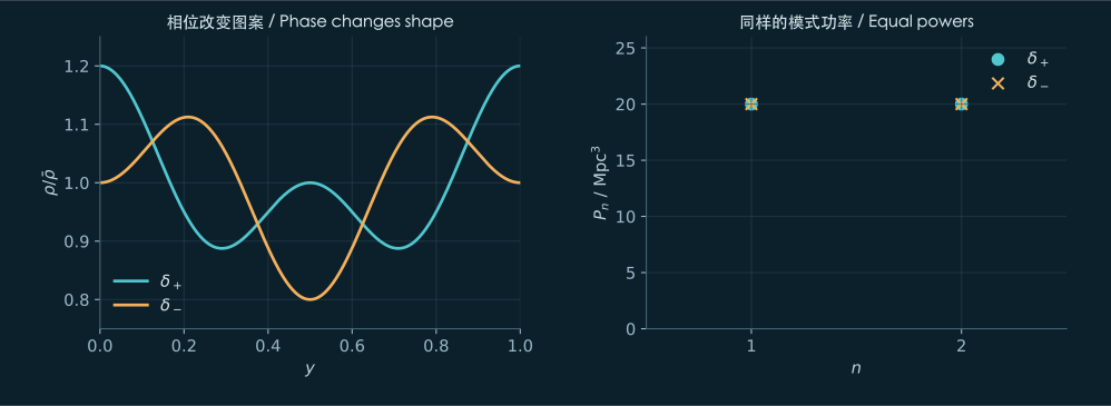
δ+(y)=0.1cos⁡(2πy)+0.1cos⁡(4πy),δ−(y)=0.1cos⁡(2πy)−0.1cos⁡(4πy)\delta_+(y)=0.1\cos(2\pi y)+0.1\cos(4\pi y),\qquad \delta_-(y)=0.1\cos(2\pi y)-0.1\cos(4\pi y)
With L=20 MpcL=20\,\mathrm{Mpc}, both positive integer modes have amplitude magnitude 0.050.05 and hence power 203(0.05)2=20 Mpc320^3(0.05)^2=20\,\mathrm{Mpc}^3.
Different positive density patterns with equal power in each of their two Fourier modes
Our analytic teaching example: change only the second wave’s sign. The density curves differ, while both n=1n=1 and n=2n=2 have 20 Mpc320\,\mathrm{Mpc}^3 power for L=20 MpcL=20\,\mathrm{Mpc}. Equal-power markers overlap at the same integer modes. This is not a PM record or a digitised paper figure. Open the full figure

Reading: Original finite-mesh calculations and independent small-wave Python replay · Springel et al., First results from IllustrisTNG: matter and galaxy clustering (2018), arXiv:1707.03397v2

Power grows faster than the amplitude

In EdS, a sufficiently small, purely growing density perturbation is proportional to the scale factor. Power is its square, so its growth ratio is the squared scale-factor ratio. Strong nonlinear evolution transfers power among waves and invalidates this simple rule.

Calculate a small plane wave first. Take initial parameter A=0.01A=0.01 and evolve from ai=0.05a_i=0.05 to af=1a_f=1. To first order, δ≃aAcos⁡(2πy)\delta\simeq aA\cos(2\pi y). The longest-mode powers are approximately 0.00050.0005 and 0.2 Mpc30.2\,\mathrm{Mpc}^3, with ratio 400400.

A finite mesh leaves a systematic difference. In the retained calibration with 16 nodes per axis and 256 steps, the actual power growth is about 0.2814%0.2814\% below 400400. More time steps alone do not remove this spatial-operator bias. Corresponding 8-node and 32-node tests are about 4.115%4.115\% and 0.02538%0.02538\% low. Particles and mesh are refined together, starting from the same continuous small wave.

P(af)P(ai)≃(afai)2\frac{P(a_f)}{P(a_i)}\simeq\left(\frac{a_f}{a_i}\right)^2
This is the small-perturbation, pure growing-mode EdS reference. The 256-step calibration differs from the Lab’s 1024-step native record; the next chapter uses an actual exported epoch.

Reading: Original finite-mesh calculations and independent small-wave Python replay · Springel et al., First results from IllustrisTNG: matter and galaxy clustering (2018), arXiv:1707.03397v2

A quiet lattice is not random sprinkling

Place four equal masses at the four quarter-interval positions of a periodic line. Their longest-mode arrows cancel exactly. The distribution is discrete, yet its power in this mode can vanish. Discreteness does not imply Poisson sampling.

Independent random points leave an average finite-sample contribution called shot noise. The TNG clustering paper discusses its subtraction and warns that cold, ordered particles can be sub-Poissonian. Our small wave begins on a regular half-cell lattice. We do not automatically subtract volume divided by particle count; that would turn a genuinely zero mode negative.

Force calculation and power measurement also differ. The force uses mesh windows, while the readout sums directly over particle positions. Taking another FFT of the displayed density would introduce its own window and aliasing, producing a different estimator.

Reading: Original finite-mesh calculations and independent small-wave Python replay · Springel et al., First results from IllustrisTNG: matter and galaxy clustering (2018), arXiv:1707.03397v2

Exercises and explained answers

  1. In the linear regime, how does doubling initial amplitude change power at a fixed epoch?

    Read the explanation

    It doubles the complex amplitude and quadruples power. Nonlinear evolution need not preserve this scaling for every late-time mode.

  2. Translate every particle by L/4L/4. What changes in the power and in the spatial pattern?

    Read the explanation

    The translation rotates each mode’s complex phase without changing its magnitude, so power stays fixed. The pattern moves in the box; its phases change consistently with that common translation.

  3. Can you subtract L3/NpL^3/N_p from a zero-power mode of the half-cell lattice?

    Read the explanation

    The independent random-sampling assumption is absent. A negative result would expose a mismatched estimator assumption, not a negative density variance.

Try the prediction

Test a small wave with full precision

  1. Select A sheet folds and reduce the amplitude to A=0.02A=0.02. Predict the early longest-mode power ratio.
  2. Pause at a saved epoch and export the current JSON, retaining its actual scale factor. Three-significant-figure readouts cannot resolve a small fractional difference reliably.
  3. Continue with the independent replay in the next chapter. Compare PM power and EdS at the same initial condition and epoch.

Sources and calculation scope

  1. Springel et al., First results from IllustrisTNG: matter and galaxy clustering (2018), arXiv:1707.03397v2

    Fixed v2: Methods 2.1–2.2 and original Figures 5–7 read. Figure 6 compares resolution and Figure 7 full-physics/DMO power; the response axes use natural logarithms. Ordered-particle shot-noise limits are discussed in Section 2.2. We inspect published methods and figures, without reproducing TNG runs or downloading snapshots.

  2. Original finite-mesh calculations and independent small-wave Python replay

    Original accepted kernel/linear, nonlinear and five-preset F64 calculations support the teaching figures and calibration. This small public ZIP contains only an exact current-state small-wave fixture, an independent NumPy/SciPy trajectory replay and expected output. The fixture was generated through the frozen model and canonical serializer in Node, not downloaded in a browser. Large raw preset archives remain separately retained; no Engine or source paper is included.

FeedbackSomething broken, confusing, or missing on this page?Tell us
What kind of feedback?

Sent with this page’s address, its Lab ID, the site language and your device type. Please leave out personal details. Feedback is kept for up to 12 months.Privacy policy