Distribute mass between the nodes
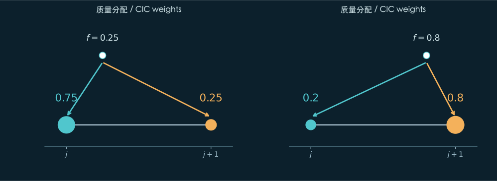
Assigning all mass to the nearest node would make the deposited field jump when a particle crossed the halfway point. Cloud-in-cell, or CIC, shares its mass between neighbouring nodes: two in one dimension and eight corners in three. The particle stays where it is; these are weights for computing a field.
Let be the fractional distance between two nodes. The left and right weights are and . A unit mass one-quarter of the way across deposits and mass units.

Reading: Springel (2005), The cosmological simulation code GADGET-2, astro-ph/0505010v1 · Original finite-mesh calculations and independent small-wave Python replay
Check mass before removing the mean
With nodes per axis and equal-mass particles, let denote the weight deposited by particle on node . Normalising by a grid volume gives density relative to the mean at the same epoch.
Adding all node masses must recover the original total. Check that first, then form the contrast . Forcing a measured mean back to unity could conceal missing periodic weights.
Reading: Original finite-mesh calculations and independent small-wave Python replay · Springel (2005), The cosmological simulation code GADGET-2, astro-ph/0505010v1
Solve the potential wave by wave
Each periodic Fourier wave has an integer vector . Its dimensionless wavenumber is , while the dimensional comoving wavenumber is . The constant, zero mode belongs to the mean background that sets expansion.
The scaled potential obeys . A second spatial derivative of a Fourier wave contributes minus its squared wavenumber, letting us solve each mode separately. CIC deposition smooths the density, and interpolating the force applies another smoothing. The declared operator explicitly corrects those two average windows.
Define , with continuous value one at zero. The window and retained modes appear below. FFT is a fast way to perform the discrete transform; the mesh and cutoff still determine its physical resolution.
Reading: Springel (2005), The cosmological simulation code GADGET-2, astro-ph/0505010v1 · Original finite-mesh calculations and independent small-wave Python replay
Bring the potential gradient back to particles
After the inverse transform, force points down the potential gradient. We use a four-point central derivative along each axis, with dimensionless grid spacing , then interpolate with the same CIC weights used for deposition.
For and , nodes are apart in comoving units, and the Fourier cutoff further limits short waves. Particles can crowd much more closely than this even though the force remains coarse. Internal details of dense knots need a separate resolution study.
Reading: Springel (2005), The cosmological simulation code GADGET-2, astro-ph/0505010v1 · Original finite-mesh calculations and independent small-wave Python replay
Kick, move, then kick again
Force changes momentum and momentum advances position. Symmetric kick–drift–kick stepping first updates part of the momentum using the old force, moves the positions, solves for their new force and completes the momentum update.
For a step from to , take , consistent with logarithmic spacing. The EdS background lets us integrate the expansion factors exactly. Write the drift and kick factors as and to distinguish them from a density growth factor.
Reading: Springel (2005), The cosmological simulation code GADGET-2, astro-ph/0505010v1 · Original finite-mesh calculations and independent small-wave Python replay
Refine time and space separately
Check the factors on an arithmetic example: to gives and . Actual trajectories divide their interval into many small steps and update density and force throughout.
At fixed mesh, doubling the step count tests temporal error in the same operator. Keeping the continuous initial condition and refining particles and mesh tests spatial and sampling errors. An independent adaptive integrator checks the former; planar collapse and linear growth also supply analytic or independent-force limits.
Mass must be conserved. Kinetic plus potential energy is generally not constant in an expanding background, and symmetric stepping alone does not prove exact energy conservation. A useful readout must still be checked under the refinement and reference appropriate to it.
Reading: Original finite-mesh calculations and independent small-wave Python replay · Springel (2005), The cosmological simulation code GADGET-2, astro-ph/0505010v1