Deform a liquid quickly, then hold its shape. Elastic memory lets stress persist and gradually relax. Hold a stress instead, and the same material can keep flowing. A spring and dashpot in series explain both responses in the Maxwell model. Two liquids with the same steady viscosity can have very different relaxation times.
Choose a shear direction and connect two elements
Take a homogeneous sample between parallel plates. The lower plate is fixed; positive horizontal displacement of the upper plate divided by the gap defines positive shear strain γ. Tangential force in that direction divided by plate area is shear stress τ. Strain is dimensionless, stress has units of pascals, and shear rate γ˙ has units of inverse seconds. This is a scalar, small-deformation, homogeneous-shear model; finite rotations require a tensor description.
The spring has shear modulus G in pascals; the dashpot has viscosity η in pascal seconds. In series they carry the same stress. Total strain adds spring strain γs and dashpot strain γd. Differentiate that sum, then replace each contribution using the two element laws. A dot denotes a time derivative.
Multiplication by viscosity gives a time in seconds, λ=η/G, called the relaxation time. It sets how quickly excess stress decays after deformation stops. Only two of modulus, viscosity and relaxation time can be chosen independently.
Start with an unstressed sample. At t=0 impose an ideal strain step γ0 and hold it. The dashpot cannot accumulate a finite strain in that instant, so the spring takes the whole step and stress jumps to Gγ0. A real instrument loads over a finite time. Its peak approaches this step result only when loading is much faster than relaxation.
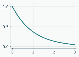
During the hold, shear rate is zero. Stress therefore changes at a rate equal to minus stress divided by relaxation time. Divide by stress and integrate: the logarithm of the stress ratio equals minus time over relaxation time. Exponentiation gives the decaying stress. One relaxation time leaves a fraction 1/e≈0.368 of the initial stress. The pure Maxwell liquid eventually relaxes to zero.
A Newtonian dashpot has no such residual stress once motion stops. An additional equilibrium spring in parallel changes the long-time result to a nonzero plateau. Then it is the excess above the plateau that follows the relaxing branch.
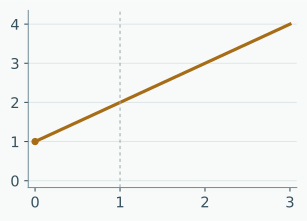
Now change the experiment. Apply and hold a stress τ0. The spring immediately contributes strain τ0/G, and the dashpot continues deforming at rate τ0/η. Total strain starts with a jump and then grows linearly. This continuing deformation is creep.
Remove the stress after a hold time th. The spring strain recovers immediately and the accumulated viscous strain τ0th/η remains. Superscripts minus and plus mean just before and just after unloading. The residual comes from viscous flow; a plastic yield law is not needed.
For G=10Pa and λ=2s, viscosity is 20Pas. A stress τ0=0.02Pa held for six seconds gives strain 0.002+0.006=0.008. Unloading recovers 0.002 and leaves 0.006. These strains are relative deformations, with no length unit.
Integrate the constant strain rate during the hold and include the spring jumps at loading and unloading. This remains an ideal step-input, small-deformation constitutive example.
A polymer solution also contains solvent. Put a Newtonian solvent element in parallel with a polymer Maxwell element: their rates are equal and their stresses add. Let solvent viscosity be ηs, polymer viscosity parameter ηp and polymer stress τp. Total model viscosity η0 is the sum, and β denotes the solvent fraction.
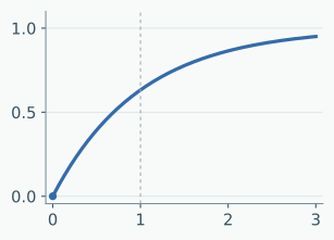
Starting from rest, step the shear rate to a constant value. Solvent stress reaches ηsγ˙ immediately; polymer stress grows exponentially from zero to ηpγ˙. This shear-stress solution also occurs in homogeneous Oldroyd-B startup shear. The next chapter introduces its normal stresses.
At steady shear the ratio of stress to rate is always η0, independent of relaxation time. Changing the relaxation time changes the approach to steady state without changing this viscosity. A steady sweep alone therefore cannot rule out material memory. This linear shear relation also does not generate shear thinning.
Solve the polymer first-order equation with zero initial stress, then add the instantaneous solvent contribution. Morozov and Spagnolie Eqs. (1.80) and (1.116) give the corresponding Oldroyd-B constitutive and steady-shear relations.
Hold strain
Vertical: τ/(Gγ0)
Horizontal: t/λ
Hold stress
Vertical: γ/(τ0/G)
Horizontal: t/λ
Start a constant shear rate
Vertical: τp/(ηpγ˙)
Horizontal: t/λ
Original analytic curves for the stated ideal protocols, not measured data. Dashed lines mark one relaxation time. Relaxation and creep start just after the ideal step. Startup shows the polymer stress alone; solvent stress is added separately.
Worked example: distinguish reported inputs from predictions
The Methods of Groisman and Steinberg’s 2000 paper report, at 12 degrees Celsius, solvent viscosity ηs=0.324Pas, solution viscosity 0.424Pas at γ˙=1s−1, and relaxation time λ=3.4s estimated from the phase shift between stress and shear rate in oscillatory tests. One viscosity point is neither a whole flow curve nor an independent zero-shear viscosity measurement.
For a single-mode teaching calculation, choose ηp=0.100Pas so the model steady viscosity matches 0.424 pascal seconds at that point. Then G=ηp/λ=0.0294Pa. Starting from rest at a shear rate of one per second, total stress begins at 0.324 pascals, reaches 0.387Pa after one relaxation time, and tends to 0.424 pascals.
To reach 99% of the polymer stress alone, solve for the exponential remainder: λln100≈15.7s. To reach 99% of the final total stress, the solvent has already supplied much of the answer. The wait is instead 10.7s. A settling tolerance needs its reference quantity.
First wait for model steady shear, then stop. Solvent stress vanishes immediately; polymer stress continues to relax. Ten seconds later it is 0.100e−10/3.4≈5.28×10−3Pa. These startup and cessation values are model predictions. Real samples can have several relaxation times, shear thinning and instrument transients; 15.7 seconds is not a universal waiting rule.
Keep deformation, observation and inertia separate
The Weissenberg number Wi multiplies relaxation time by a characteristic shear rate. It compares memory with deformation. The Deborah number De instead compares relaxation time with a chosen observation duration Tobs. A long observation can still contain rapid sustained shear. The two comparisons answer different questions.
Check inertia using the Reynolds number, with speed U, length L, density ρ and a stated viscosity, here the total model value η0. Only after choosing shear rate as speed over size does their ratio take the form below. A larger ratio makes elasticity more important relative to inertia; it does not by itself make elastic stress large.
Our example has Wi=3.4. That does not specify every elastic-to-viscous stress ratio or establish an instability threshold: polymer share, flow and geometry matter. Groisman and Steinberg report the same normalized resistance relation after reducing every apparatus dimension fourfold at equal shear rate. Speed fell fourfold and Reynolds number sixteenfold. This supports their low-inertia elastic-instability interpretation; the paper says the rescaled data are not separately plotted. The scalar Maxwell equation does not itself predict that instability.
The first definitions compare deformation, observation and inertia. The last relation additionally assumes the shear-rate scale is speed divided by length.
Choose Viscoelastic hold and predict whether stress will reach zero. This is a tensile specimen with an equilibrium spring parallel to one Maxwell branch, so a nonzero plateau remains.
Set each hold to ten seconds and Maxwell relaxation time to one second. Find the excess stress above the plateau at hold onset, then the point at 1/e of that excess. They should be about one second apart. Compare excess stress, not total stress.
Change relaxation time to five seconds. Predict how much excess disappears during a ten-second hold, then inspect the curve. Loading is a finite ramp, so its rate also changes the starting peak.
Use Newtonian standard and record torque and apparent viscosity at two speeds. Then choose Shear thinning. Predict which quantity can rise and which can fall.
This rheometer gives isothermal, no-slip, memoryless steady readings from the current shear rate. It has no relaxation time; matching viscosity values do not replace a relaxation measurement.
For the example’s Maxwell-plus-solvent model, calculate separate waits for 99% of polymer stress and 99% of total stress. Explain the difference between about 15.7 and 10.7 seconds.
Exercises with explained answers
A pure Maxwell liquid with G=10Pa and λ=2s receives an ideal strain step of 0.005. Find stress immediately and after four seconds.
Show the answer
Initially Gγ0=0.05Pa; after four seconds 0.05e−2≈0.00677Pa. Two relaxation times leave about 13.5%. These values assume the ideal step.
Hold the same liquid at a shear stress of 0.02 pascals for six seconds, then unload. Which strain recovers and which remains?
Show the answer
Viscosity is twenty pascal seconds. Spring strain is 0.002 and accumulated dashpot strain is 0.006, for a total of 0.008. The spring recovers 0.002 on unloading; the viscous strain of 0.006 remains.
Two Maxwell liquids have the same viscosity but relaxation times of one and ten seconds. Can steady shear alone distinguish them?
Show the answer
No. Their steady stresses equal the same viscosity times the shear rate. Startup, cessation or oscillation can distinguish the time response. The longer-relaxing liquid loses an initial stress more slowly.
Reduce every apparatus dimension tenfold at fixed fluid and shear rate. What happens to Reynolds and Weissenberg numbers? Does that alone establish instability?
Show the answer
Weissenberg number is unchanged. Speed and length each fall tenfold, so Reynolds number falls a hundredfold. Inertia is smaller, but material, flow and boundary conditions still determine instability; the ratio alone is insufficient.
Section 3: the Weissenberg number defined as the relaxation time times the shear rate, and Eq. (1.27), the generalized Newtonian liquid. Section 4.1: Eqs. (1.47)–(1.51), the spring, the dashpot, the Maxwell liquid and its memory integral, with a relaxation time equal to viscosity over modulus. Eq. (1.72): the upper-convected derivative; Eq. (1.80): Oldroyd-B; Eqs. (1.86)–(1.87): FENE-P. Section 4.4: the Hookean dumbbell, Eqs. (1.98)–(1.110). Eq. (1.116): the steady-shear normal stress of Oldroyd-B. Eqs. (1.117)–(1.125): hoop stress and the cone-and-plate normal force. Eqs. (1.128)–(1.131): uniaxial extension and the Oldroyd-B divergence at half the inverse relaxation time. The chapter has no startup solution and no planar extension; the course derives both.
arXiv version 1, read in full. Fig. 1: swirling flow between a rotating plate of radius 38 mm and a cup of radius 43.6 mm, liquid depth 10 mm, 12 °C. Methods: 65 % saccharose and 1 % NaCl solvent of viscosity 0.324 Pa s with 80 ppm polyacrylamide of molecular weight 1.8e7; solution viscosity 0.424 Pa s at a shear rate of 1 per second; relaxation time 3.4 s. Fig. 2: transition near a shear rate of 1 per second (Weissenberg number 3.5, Reynolds number about 0.3), with hysteresis; resistance up to about 12 times laminar for a 10 mm gap and 19 for 20 mm. Fig. 3: snapshots at Weissenberg number 13. Fig. 4: brightness spectra. Fig. 5: velocity spectra, a power law with exponent −3.5 at 4 per second over about one decade. Text: Reynolds stress below 0.5 % of the resistance.
Keep reading
What this page links to directly
You are hereStress relaxation and creep in a Maxwell liquid