Why averaging magnitudes fails
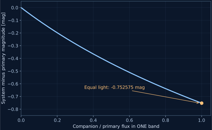
Replace one lamp with two identical lamps and the receiving surface gets twice the light. Flux adds directly. Magnitudes take a logarithm of flux so a large brightness range fits on a convenient numerical scale. Numbers that have already been logged cannot be added as though they were the original light.
In band , let be the magnitude-system zero-point flux. Absolute magnitude refers to placing the source at ten parsecs. Its flux ratio follows the definition below.
Two identical components make a system approximately 0.752575 magnitudes brighter than either one. This number follows from the logarithmic definition, not a stellar-evolution parameter. Adding component birth masses does not justify looking up their summed mass as one single star. A single star with twice the mass has its own structure and luminosity.
Reading: Kroupa (2001), On the variation of the initial mass function · Reyes et al. (2024), a precise M67 isochrone; native ISOA data
Finish each band before taking a colour
The Lab uses native G, BP and RP magnitudes. Look up each component’s three absolute magnitudes, combine the light within each band, and only then subtract RP magnitude from BP magnitude. Two BP flux ratios can be added, as can two RP ratios. BP and RP have different zero points, so adding their dimensionless ratios does not yield total physical energy.
For a checkable example, give the first component G, BP and RP absolute magnitudes of 4, 5 and 3, and the second 6, 7.5 and 5. The combined values are approximately 3.840270, 4.896518 and 2.840270. The resulting colour is approximately 2.056248, not the arithmetic mean of the component colours.
The public default takes magnitudes directly from 98 licensed native nodes. Local models interpolate mass only within a valid, equal-source-phase interval. Different phase labels refuse the bridge. If either component of a pair lacks support, the complete three-band system light is marked unsupported. That flag describes table support; the real component’s luminosity remains undetermined here.
Reading: Reyes et al. (2024), a precise M67 isochrone; native ISOA data · PARSEC/CMD3.8 official input help and phase labels · MIST official isochrone interface and user documentation
Distance belongs to the system’s position
A cluster has depth. Put an observer at a fixed direction behind its centre, and describe every system with three coordinates relative to that centre. All three enter its distance to the observer. Using the central distance for every component would discard the geometry we just assigned.
This distance modulus follows from the inverse-square decline of received light. Moving the same system farther away adds the same magnitude shift in every band. Without extra extinction its colour stays fixed. Doubling distance adds approximately 1.50515 magnitudes. A brightness limit can then remove the system, changing the selected sample indirectly.
The record retains position, actual distance, component IDs and band light. The screen marker has compressed brightness and size so members remain visible. Distance always comes from the physical parsec coordinates.
Reading: Gaia DR3 documentation and archive
An aperture selects a cone
A telescope accepts an angular field. Different depths on the same line of sight therefore have slightly different allowed transverse radii. The green ring is the intersection with the cluster-centre plane. It does not turn the three-dimensional cone into a cylinder of fixed physical radius.
A projected radius of 5 pc at a forward distance of 1000 pc subtends approximately 0.2865 degrees. An aperture of 0.2 degrees excludes it; 0.3 degrees includes it if the light also passes the magnitude limit. Neither operation moves the star or changes its age.
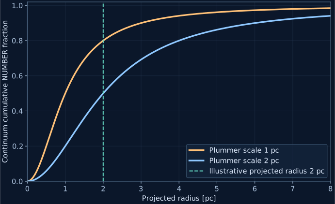
The radial chart uses projected physical radius from the cluster centre and separately accumulates supported system number and apparent G light. Its green line marks the aperture radius at the central plane. Actual selection still calculates every system angle. The line is not an exact physical-radius cut at every depth, and both cumulative curves refer only to systems with complete photometric support.
Keep one record all the way through
An observed synthetic point can now be traced back: which components it contains, which native mass or valid interpolation interval supplies their light, how G light adds, where the system lies, how far it is, and why it passes or fails selection. The scene, diagram and export carry the identities and calculated quantities of that same population.
These light predictions use several specific assumptions. Random pairing supplies no physical binary orbit or interaction. Concentration is imposed. A sharp magnitude limit is not a complete detection-efficiency model. Real data also need errors, field contamination and an extinction distribution. This model predicts what follows from stated assumptions; it does not invert the sky into parameter probabilities.
Reading: Reyes et al. (2024), a precise M67 isochrone; native ISOA data · Gaia DR3 documentation and archive