Start with one unexpectedly bright point
Imagine a photograph of a star cluster. One point has nearly the colour of a neighbouring star but is noticeably brighter. It may be a more luminous individual star. It may also contain two stars whose images the telescope cannot separate. An unresolved binary is still two physical components; the observation blends their light into one point.
Two identical components at the same distance deliver twice the light without changing the colour. Astronomers record brightness with magnitudes, whose numbers decrease as an object becomes brighter. Doubling the light makes the combined point about 0.75 magnitudes brighter. A population with exactly one age can therefore have points above its single-star sequence. Unequal components can also change the colour because they contribute different proportions in different bands.
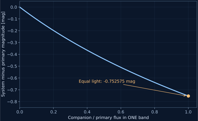
This illustration calculates light addition. It does not calculate a binary orbit, mass exchange or a merger. Those are separate physical questions. Here we can settle one useful piece completely: given two components, where does their combined light go?
Reading: Kroupa (2001), On the variation of the initial mass function
One age still leaves many birth masses
Separating every binary would not collapse the cluster to one point. Stars begin with different masses. Mass affects internal pressure and temperature, nuclear energy generation and the surface that radiates that energy. More massive stars generally spend their available central fuel faster. After a shared interval, some components still burn hydrogen in their centres while others have left that stage.
A common age fixes elapsed time, not birth mass. For a stated composition and age, a stellar model predicts a position for each initial mass. The resulting model curve is an isochrone. It is not a line drawn through whatever points happen to be in a photograph, and equal lengths along it do not represent equal numbers of stars. Their numbers require a birth-mass distribution and a selection rule.
The public Lab uses one expressly licensed model at 3.95 Gyr. Its selected hydrogen-burning subset has 98 native mass nodes between approximately 0.851 and 1.262 solar masses. It does not invent lower-mass companions, giants or remnants outside that support. The default therefore describes the light of a restricted conditional population, not the complete M67 cluster.
Reading: Reyes et al. (2024), a precise M67 isochrone; native ISOA data
A colour requires two measurements
Blue and orange markers are convenient, but a research colour needs a defined observation. Measure light through one passband, measure it through another, and compare the results. A passband specifies which part of the spectrum the instrument accepts. Surface temperature changes how a star distributes its light between those bands.
To blend a pair, add its component light separately within each band and then calculate the colour. Averaging two magnitudes or two colours gives the wrong operation. A cool companion may add an appreciable amount of red-band light while contributing very little in a blue band.
The Lab compresses marker brightness so faint members remain visible, and uses colour as an ordered cue. These markers are not calibrated display RGB or actual stellar radii. The charts and saved record use the computed band magnitudes. The public default uses Gaia DR2 passbands; the named local models use EDR3. Their labels change with the model, and their similar names do not justify mixing them.
Reading: Reyes et al. (2024), a precise M67 isochrone; native ISOA data · MIST official isochrone interface and user documentation
Change the field, change the sample
A smaller telescope field removes members from the diagram. If more massive systems are concentrated near the centre, a narrow field can retain a large share of the bright light while excluding many outer systems. The measured brightness distribution changes although every birthday stays fixed.
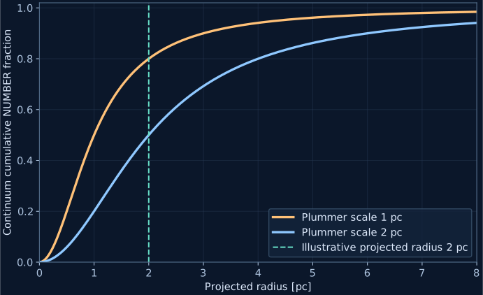
The green aperture ring represents a physical angle around the fixed observing direction. Dragging it selects the same system IDs in the scene, diagram and export. The model also carries each system’s own three-dimensional position into its distance from the observer. Orbiting the display camera changes the view of the model, not the telescope selection.
The degree of massive-system concentration is imposed here. It is a spatial snapshot, not the result of evolving gravity for an elapsed time. The original cluster mode has its own separate N-body clock. Explaining a real concentration requires comparing formation, gravitational rearrangement, selection and subsequent stellar evolution.
Width begins an investigation
A broad diagram now gives several concrete checks. Ask which component masses were drawn, how their light was combined and which systems reached the selected sample. In real observations, foreground extinction, measurement errors and unrelated field stars can add further width. Their omission from this small model does not remove them from the sky.
If those effects cannot explain the observations, propose age or composition differences and calculate predictions that distinguish them. Width alone does not measure an age spread. Chemical multiple populations require evidence about element abundances, beyond a second ridge of blended light.
The following chapters trace the same observation in order: draw component masses, combine the components into one point, and check where a native age curve has support. Each step can be changed independently and leaves a record of what was actually calculated.