Draw masses before counting stars

A bin count depends on its width

Start with a histogram of birth masses. A bin from one to two solar masses is half as wide as a bin from two to four. Equal counts in those bins do not imply equal numbers per unit mass. The horizontal coordinate matters before we interpret a slope.

Write birth mass in solar units as $m=M_{\rm birth}/M_\odot$ and let $\xi(m)\,dm$ be the expected component count in a narrow interval. This initial mass function, or IMF, describes a distribution across possible populations. One draw of 1024 components need not equal its expected count in every bin.

\Pr(a<m<b)={\int_a^b\xi(m)\,dm\over\int_{m_{\min}}^{m_{\max}}\xi(m)\,dm}

The numerator adds the target mass bins; the denominator adds the entire supported interval. Their ratio is a component probability.

A logarithmic horizontal axis changes the actual mass width of an equally wide plotted bin. A number density per mass and a number density per log mass therefore have different slopes even when they describe the same stars.

Reading: Kroupa (2001), On the variation of the initial mass function

A finite broken power law

The local twelve-age models use a stated teaching family from 0.1 to 8 solar masses, with a break at 0.5. It contains many light components and fewer massive ones. This is not an IMF recovered from M67, and the truncation makes no claim that stars outside it do not exist.

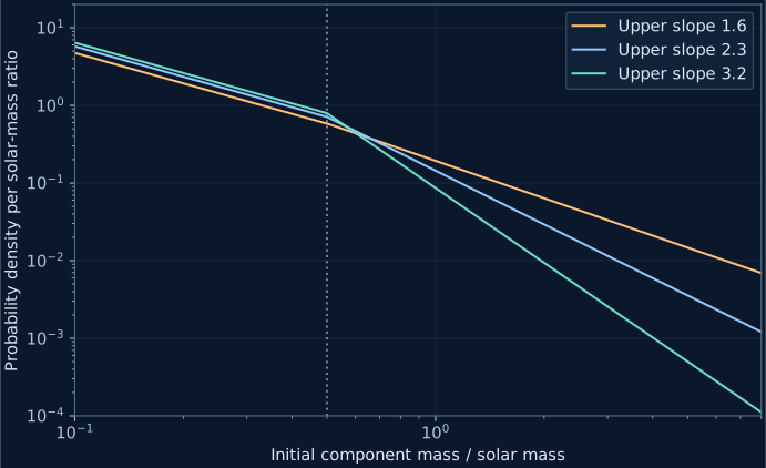
\xi(m)\propto\begin{cases}m^{-1.3},&0.1\le m<0.5,\\0.5^{\alpha-1.3}m^{-\alpha},&0.5\le m\le8.\end{cases}

The prefactor joins the branches at 0.5. Normalization still requires the total finite-interval area. Increasing the high-mass slope reduces the relative number of massive components.

Own finite broken component-mass probability densities for three upper slopes — Own analytic teaching distributions on0.1–8 solar masses, normalized per unit mass ratio. The public fixed-age model instead conditions on its much narrower native support and samples discrete nodes.

For a single slope $a$ , integrate between lower mass $l$ and upper mass $h$ . At slope one the familiar quotient appears singular, but its limit is a logarithm.

I_a(l,h)=\begin{cases}\dfrac{h^{1-a}-l^{1-a}}{1-a},&a\ne1,\\[4pt]\ln(h/l),&a=1.\end{cases}

The logarithm is natural. A stable implementation uses the logarithmic limit near slope one instead of subtracting almost equal numbers.

As an independent example, restrict the distribution to 0.5–2 solar masses with slope 2.3. The probability between 1 and 2 is approximately 0.288826. In 1024 independent draws, the expected count is about 296 and its standard deviation about 14.5. Counts of 282 or 307 do not by themselves indicate a faulty sampler. This arithmetic example has a different mass support from the public default.

Reading: Kroupa (2001), On the variation of the initial mass function

Turn a uniform draw into a mass

Imagine a strip from zero to one. Its left part represents the probability of the lower branch and its right part the upper branch. A uniform draw first chooses a branch. Within it, invert the accumulated area to find a mass. There is no need to guess masses repeatedly until one is accepted.

m(u)=\begin{cases}\left[l^{1-a}+u\left(h^{1-a}-l^{1-a}\right)\right]^{1/(1-a)},&a\ne1,\\l(h/l)^u,&a=1.\end{cases}

This inverse cumulative distribution sets the integrated fraction below the mass equal to the uniform number and solves for mass. A broken law first selects a branch by its total area, then remaps the uniform draw within it.

Save the seed and the actual mass list. A seed makes a sample reproducible; it does not turn that sample into a population average. Validation also has two distinct questions: whether the deterministic CDF calculation is correct, and how far one random sample lies from it. A sample can occasionally cross a prespecified statistical bound. The tutorial retains one such failure.

Reading: Kroupa (2001), On the variation of the initial mass function

When the source supplies 98 native nodes

The licensed public model supplies only a fixed-age set of 98 selected nodes. We first tested continuous mass draws followed by linear photometric interpolation. With alternating source rows withheld, the maximum magnitude discrepancy was 0.003018, beyond the prespecified 0.002 exploratory gate. That failure remains recorded; the public default does not use this continuous photometry branch.

Instead, place cell boundaries at adjacent mass midpoints and at the two support endpoints. Give native node $i$ the probability contained in its mass cell. Drawing a cell selects that original node mass and its original band magnitudes. No intermediate luminosity is invented.

w_i={\int_{b_{i-1}}^{b_i}\xi(m)\,dm\over\int_{m_{\min}}^{m_{\max}}\xi(m)\,dm},\qquad\sum_iw_i=1

These are midpoint cells in mass, not equally weighted row indices. Every weight is positive and the cells partition the stated mass support.

The result is a mass-discretized conditional population. It preserves the integrated number probability of each cell, but the discrete mean mass need not equal the continuous IMF mean exactly. The saved birth mass must be the sum of the nodes actually drawn. Equal probability per native row would introduce an additional, unjustified bias because the node spacing is unequal.

Reading: Reyes et al. (2024), a precise M67 isochrone; native ISOA data

Draw components before making companions

Drawing a primary and then appending a companion would change the component mass distribution just specified. Here all 1024 components are drawn first. Their IDs are randomly permuted, some are paired, and the rest remain singles. Every ID is used once.

N_{\rm pair}=\left\lfloor {f_bN_c\over1+f_b}\right\rfloor,\qquad N_{\rm sys}=N_c-N_{\rm pair}

Solve for pair count from the requested binary-system fraction and fixed component count, then round down. The fraction denominator is systems, not components.

For a requested fraction 0.35 and 1024 components, there are 265 pairs and 759 systems. The realized binary-system fraction is approximately 0.349144. The rounding difference remains in the readout. Summed system birth masses must equal summed component masses. This mass conservation concerns the same drawn components. Changing the mass-distribution slope can change their total drawn mass.

Random pairing is a declared choice, not an empirical binary mass-ratio law. The next chapter takes this same saved list and calculates the light each unresolved system actually contributes.

Reading: Kroupa (2001), On the variation of the initial mass function

Draw masses before counting stars

A bin count depends on its width

A finite broken power law

Turn a uniform draw into a mass

When the source supplies 98 native nodes

Draw components before making companions

Exercises and explanations

Try the prediction

Account for every component

Change counts on fixed nodes

Sources and calculation scope