Recalculate a point blast and read the fixed HESS 2004 spectrum

Start in an empty directory

Download the scientific ZIP below and extract it into a new directory. Read README.md and input-lineage.json before running. The package contains independent Python producers and their own inputs. Its default command verifies the file inventory and performs five numerical steps with no network or cached completed result.

The first step integrates the n7 and n12 ejecta-envelope shells at two tolerances. The second independently integrates the zero-ejecta point blast at three central cuts. The third uses the freshly calculated n7 coefficients in five passive acceleration cases and five deliberately rejected or energy-limited examples. The fourth calculates the angular mean-log discrepancy. The fifth draws three synthetic scientific figures.

Open replay-receipt.json and the individual logs. Each calculation writes a new output. The reader’s registered particle cases have their own physical ages, whereas the interactive density study holds one age fixed. The two sets serve different finite tests.

python3 replay.py --output /absolute/new/remnant-run

Reading: Sandbox Physics independent supernova-remnant Python science reader

Recover the point-blast coefficient from energy

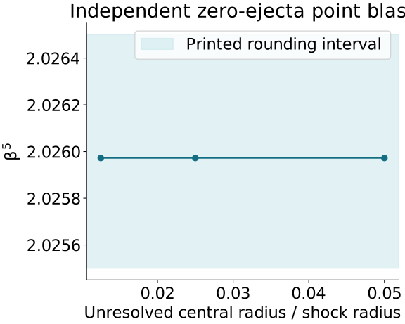
Open point-blast/results.json. Each run reports its central cut, resolved energy, estimated central thermal contribution, swept-mass error and a local energy-flux check. In units where shock radius, age and ambient density are one, the dimensionless energy integral $I$ fixes $\beta=I^{-1/5}$ .

Compare the three cuts $0.05,0.025,0.0125$ . The result approaches $\beta^5\simeq2.0259724$ , within the original rounded coefficient interval. The code does not rescale the profile afterward to manufacture the energy. The central approximation is exposed through the shrinking-cut comparison.

As a worked unit check, $E/\rho_0$ has units $\mathrm{m^5\,s^{-2}}$ . Multiplying by age squared gives $\mathrm{m^5}$ , and a fifth root gives a radius. Increasing age by a factor of four therefore increases radius by $4^{2/5}\simeq1.741$ . This scaling belongs to the separate zero-ejecta problem.

Own point-blast coefficient compared at three decreasing unresolved central radii with the printed rounding interval. — Own newly integrated point-blast results. The shaded interval represents rounding in the cited coefficient, not an observational confidence interval.

Reading: Leahy & Williams (2017), A Python Calculator for Supernova Remnant Evolution, arXiv1701.05942v2 · Sandbox Physics independent supernova-remnant Python science reader

Obtain exactly the historical whole-remnant table

For the optional exercise, open Aharonian et al., A detailed spectral and morphological study of the gamma-ray supernova remnant RX J1713.7−3946 with HESS, arXiv astro-ph/0511678v2, published in Astronomy & Astrophysics 449, 223–242 (2006). The measurement used here is the 2004 whole-remnant spectrum in Figure 12, not a 2006 observing campaign or the later deep HESS spectrum.

Section 3.2 identifies a $0.65^\circ$ radius aperture and 30.5 hours of selected live time for this spectrum. The exact official auxiliary HTML has 9734 bytes and SHA256 shown in the package README. The optional command fetches only that object, verifies all its bytes, extracts 25 rows and creates the local figure hess2004-private.png. Original data and that derived image stay in your private output directory.

The eight table columns are row number, energy centre, lower energy edge, upper edge, differential photon flux, lower statistical uncertainty, upper statistical uncertainty and a systematic percentage. The code checks consecutive row numbers, positive finite values, centres inside bins and adjoining bin edges before analysis. Changing one source byte causes refusal before creating an analysis directory.

python3 optional_observed.py --fetch --output /absolute/new/private/hess-run

Reading: Aharonian et al. (2006), A detailed spectral and morphological study of RX J1713.7−3946 with HESS, astro-ph/0511678v2 · Official HESS auxiliary page for the historical Figure12 whole-remnant spectrum · Sandbox Physics independent supernova-remnant Python science reader

Read the photon flux before choosing a model

Energy is in TeV. Differential photon flux has units $\mathrm{TeV^{-1}\,cm^{-2}\,s^{-1}}$ : photons per energy, collecting area and time. Multiplying by $E^2$ makes an energy-flux display per logarithmic energy interval. Converting its remaining TeV to erg uses $1\,\mathrm{TeV}=1.602176634\,\mathrm{erg}$ .

The two models in this exercise are a power law and that same power law multiplied by $e^{-E/E_c}$ . The normalization is defined at 1 TeV, and $\Gamma$ is the photon index. It describes the photons; it is not automatically the momentum index of accelerated protons.

The original Figure 12 also contains other instruments and years. Extracting only the named 2004 table avoids mixing apertures and epochs. The original Figure 13 and Table 1 compare several curved spectral shapes; a cutoff is not the only phenomenological description that the paper finds acceptable.

F(E)=N\left(\frac{E}{1\,\mathrm{TeV}}\right)^{-\Gamma}\exp(-E/E_c)

Removing the exponential gives the power-law model.

N

retains the differential photon-flux units.

State the fit approximation and keep its failed test

The point-centre fit evaluates the model at each published energy centre. A diagonal Gaussian approximation divides each residual by its quoted statistical uncertainty, then sums the squares. For an asymmetric error bar, this calculation uses the lower uncertainty when the model lies below the point and the upper when it lies above. Correlations and the original event response are not reconstructed.

For example, suppose a point is 5 in some flux unit, its lower error is 1 and upper error 2, and a model predicts 6. The chosen residual is $(6-5)/2=0.5$ , contributing 0.25 to chi-square. The piecewise error choice is part of the approximation, not a new instrument likelihood.

The 25 points leave 23 degrees of freedom for the two-parameter power law and 22 for the three-parameter cutoff. The point-centre power law gives $\chi^2=88.6192$ compared with the published 85.6. The difference 3.0192 exceeds the predeclared 2.0 comparison threshold. That test fails, even though the best-fit parameters lie within the published one-standard-deviation intervals.

A second calculation averages the model uniformly over each published energy bin using 32 positive Gauss–Legendre nodes. Its independent analytic or adaptive-integral check passes, but the power-law chi-square becomes 89.5348; its difference 3.9348 still fails the same threshold. Uniform bin averaging does not restore an unavailable response-weighted analysis. Both original failed results are retained.

The point-centre cutoff gives $\Gamma\simeq1.9723$ and $E_c\simeq11.3614\,\mathrm{TeV}$ , with $\chi^2\simeq28.0347$ for 22 degrees of freedom. The published values are 1.98, 12 TeV and 27.4. The curvature comparison is informative within this approximation, but exact reproduction of the original fitting procedure has not been achieved.

\chi^2=\sum_i\left[\frac{F_{\rm model}(E_i)-F_i}{\sigma_i}\right]^2,\qquad \overline F_i=\frac{1}{E_i^+-E_i^-}\int_{E_i^-}^{E_i^+}F(E)\,dE

These are two declared high-level approximations. A successful expected-failure replay means the failed comparison was reproduced, not that its original threshold was passed.

Reading: Aharonian et al. (2006), A detailed spectral and morphological study of RX J1713.7−3946 with HESS, astro-ph/0511678v2 · Sandbox Physics independent supernova-remnant Python science reader

Move the energy scale as one shared uncertainty

The original discussion gives an approximately 20 percent common energy-scale uncertainty. If every photon energy is shifted by factor $s$ , conservation of photon counts requires differential flux and its errors to divide by $s$ . Moving only the horizontal coordinates would change the represented photon number.

For the cutoff model, this transformation gives $E_c\to sE_c$ , leaves $\Gamma$ unchanged and changes the 1 TeV normalization by $s^{\Gamma-1}$ . The reader actually refits scale factors 0.8 and 1.2 and checks this relation. It is a correlated systematic scenario, not 25 independent random errors.

A reusable checklist is to identify the observing epoch and aperture, read the units and bin edges, state the fit and error model, distinguish common calibration shifts from point errors, and keep every failed comparison visible. Before inferring a parent-particle population, add the radiation process, target material and corresponding response analysis.

E'=sE,\qquad F'(E')=\frac{1}{s}F(E'/s)

The Jacobian preserves the photon number integrated over corresponding energy intervals.

Reading: Aharonian et al. (2006), A detailed spectral and morphological study of RX J1713.7−3946 with HESS, astro-ph/0511678v2 · Sandbox Physics independent supernova-remnant Python science reader

Exercises and explanations

A wrapper exits successfully after reproducing an expected chi-square failure. Has the published chi-square agreement passed?
Read the explanation
No. The wrapper has checked that the source identity and calculation reproduce the registered failure. The original 2.0 difference threshold remains failed and is reported separately.
Why does a $20\%$ common energy-scale shift not belong in 25 independent vertical error bars?
Read the explanation
The same calibration change moves every energy and differential-flux value coherently. Treating it as independent point noise would allow mutually inconsistent shifts and change the assumed statistical model.
Can the fitted gamma-ray photon index be inserted directly into the mean-cycle proton plot?
Read the explanation
No. A photon spectrum depends on the emitting particle distribution and radiation mechanism, including target gas or photon fields. The passive cycle model has not calculated that emission.

Try the prediction

Compare a saved particle record with a photon table

Export a complete accepted particle record and identify its momentum unit, weights and short clock window.
Run the default offline reader and inspect the independent point-blast mass and energy checks.
Run the optional historical photon exercise separately. List the additional physical ingredients needed to predict those photons from a particle population before comparing their indices.

Standalone scientific materials

Download the scientific ZIP · Read the setup and calculation scope

The standalone ZIP recomputes own gas solutions and passive particle cycles with zero network. The optional historical exercise obtains one exact HESS table locally, generates its private plot and preserves both failed chi-square comparisons. No app, original paper or observation is bundled.

Sources and calculation scope

Leahy & Williams (2017), A Python Calculator for Supernova Remnant Evolution, arXiv1701.05942v2
Selected sections3.2.1/3.3.3 and printed coefficient on page16. The own Euler point-blast integral is independently recalculated; only these source sections, not the complete paper, are claimed read. TM99 full text was not acquired.
Aharonian et al. (2006), A detailed spectral and morphological study of RX J1713.7−3946 with HESS, astro-ph/0511678v2
Fixed historical 2004 whole-remnant Figure12, sections2.5.2/3.2 and Table1. Selected original methods/results read; no original event/response reconstruction. Both point-centre and finite-bin chi-square comparison failures are retained.
Official HESS auxiliary page for the historical Figure12 whole-remnant spectrum
Exact9734-byte HTML, complete SHA in the reader setup;25 named high-level photon rows. Optional reader acquires it locally. Original table and observation-derived plots are not redistributed.
Sandbox Physics independent supernova-remnant Python science reader
Own offline Euler n7/n12, independent zero-ejecta point blast, mean cohorts, angle/first-passage/Jensen checks and synthetic plots. Recalculates fresh coefficients and all default steps; original papers/data and app/Engine code excluded.