Read the two axes before the curve
The Hertzsprung–Russell diagram compares surface effective temperature with luminosity. Effective temperature is the temperature a blackbody would need to emit the same surface energy flux. Luminosity is the total energy emitted per second. In the conventional diagram, hotter stars lie to the left and more luminous stars higher up.
The surface quantities are related by , where is photospheric radius and is the Stefan–Boltzmann constant. A star can become more luminous while its surface cools if its radius increases sufficiently. Surface colour alone does not reveal the core temperature.
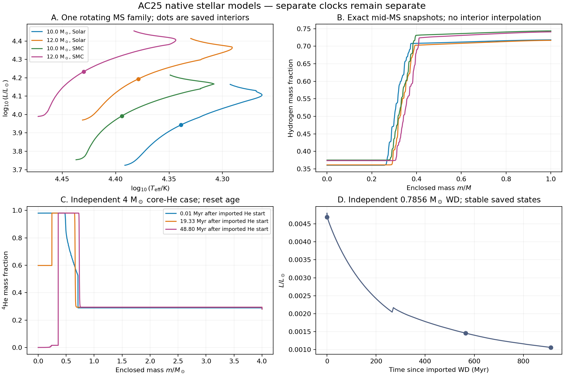
The atlas draws each model’s own history curve and marks its selected saved interior in gold. A file called profile3 is the third saved profile, not necessarily stellar model number three. Match the header and index before attaching a physical interpretation to a point.
Sources: MESA 25.12.1, history, profile and restart output documentation · Keszthelyi (2022), fixed reproduction package, Zenodo 7069766, CC BY 4.0
Count hydrogen inside the actual shells
Let be the hydrogen mass fraction of a shell. Multiply that fraction by the shell mass, then sum over the star. This gives the total mass of hydrogen still present. In an enclosed-mass profile, successive mass boundaries supply the shell masses.
A drop in the total hydrogen mass has two possible contributions in a wind-losing star: nuclear consumption and hydrogen carried away with the wind. To estimate nuclear consumption, subtract the wind contribution. The surface hydrogen fraction weights the matter that leaves.
Use the accepted physical time intervals. In the selected massive-star files, the current row’s mass-loss rate belongs to the interval ending at that row. Summing those recorded step contributions reproduces the total lost mass. A trapezoid is a different quadrature rule and gives a visibly different answer for the small wind loss.
Sources: Keszthelyi (2022), fixed reproduction package, Zenodo 7069766, CC BY 4.0 · MESA 25.12.1, history, profile and restart output documentation
From fuel to an energy scale
Hydrogen-to-helium fusion releases binding energy because the final particles have a smaller total rest mass. Some released energy leaves in neutrinos. The nuclear heating available to the gas therefore depends on the reaction network and on the convention used for neutrino losses.
The independent ten-solar-mass Solar-composition calculation gives about of integrated H-burning heat per gram consumed over its recorded main-sequence interval. The total atomic mass-defect ceiling is about . The lower heating value is physically plausible; the ceiling is not a replacement for a complete network calculation.
For a worked scale estimate, that track burns about of hydrogen after correcting for the wind. Multiplying by its heating per gram gives roughly . Dividing by about gives a mean H-burning luminosity near .
That is a nuclear heating estimate. A complete energy calculation must also account for stored internal energy, gravity, neutrinos and any energy carried through a changing boundary. That global comparison requires additional time-resolved energy terms absent from the saved massive-star subset. The fuel integral here measures the hydrogen consumed and the heat released per gram.
Sources: Keszthelyi (2022), fixed reproduction package, Zenodo 7069766, CC BY 4.0 · NIST atomic masses, hydrogen isotopes · NIST atomic masses, helium isotopes · Jermyn et al., MESA VI, arXiv:2208.03651v2, Section V energy consistency
The central mixture changes before the envelope is empty
The main-sequence core converts hydrogen into helium. Its mean particle mass changes, and the pressure, temperature and burning rate readjust. Core mixing can keep part of the composition nearly uniform, while the surrounding layers develop a chemical gradient. The star’s surface position moves as the entire structure responds.
Within the fixed Solar-composition family, the recorded core-H interval is shorter for the initially twelve-solar-mass star than for the ten-solar-mass star. The table measures the interval after the source’s operational ZAMS and before its final retained core-H point; it is not the complete time since formation.
Once central hydrogen is exhausted, hydrogen can still burn in a shell around a contracting helium-rich core. The envelope can expand as the thermal structure changes, lowering the surface temperature. To identify a later turn on the HR track, inspect its burning and composition profiles. The bend itself supplies two surface coordinates.
| Initial mass | Recorded core-H interval | Fixed model family |
|---|---|---|
| Solar composition, NOMAG/Mix1 | ||
| Solar composition, NOMAG/Mix1 |
Sources: Keszthelyi (2022), fixed reproduction package, Zenodo 7069766, CC BY 4.0 · Keszthelyi et al., arXiv:2209.06350v1, rotating stellar grids and physical prescriptions · Dotter (2016), MIST 0, arXiv:1601.05144v1, phase-aware track interpolation
Helium burning builds a different core
The separate four-solar-mass example begins from an imported core-He-burning structure. Its clock is reset at that point. It is a new case, not the continuation of either massive-star track above.
At the first saved state the central helium fraction is about 0.98. In a middle state it is about 0.60; by the final state it is close to exhaustion. Helium reactions make carbon, and reactions involving helium and carbon also build oxygen. The saved carbon and oxygen profiles reveal where those products accumulate.
Hydrogen burning can continue in a surrounding shell at the same time. Surface luminosity should therefore not be assigned entirely to the central helium reaction. The separate source columns show how much power each burning process supplies.
The envelope also readjusts. Across three of the saved He-burning states, the photospheric radius changes from about forty-two solar radii to twenty-two and then thirty-two. The corresponding surface temperatures and luminosities make an HR curve with a changing direction. The last saved state reaches terminal core-He burning. Further calculations would be needed to follow this case toward a remnant.
A white dwarf shines mostly by losing stored energy
The independent cooling case is an already formed white dwarf of . It contains a carbon–oxygen-rich interior and a thin helium-rich outer region. Its imported-model clock does not include a progenitor lifetime or determine the progenitor’s initial composition.
In the supported saved states, nuclear heating is tiny compared with the surface luminosity. The remnant can still resist gravity through electron degeneracy pressure while it loses stored energy. Mechanical support and the energy supply for the light are different parts of the problem.
Its luminosity falls from about at the first supported snapshot to at the final one. The radius remains close to one hundredth of a solar radius. These native states illustrate a compact remnant cooling. The sparse energy outputs leave a measured late global discrepancy, so the displayed ages retain the source’s clock and its limits.
Sources: Kumar and Townsley (2025), fixed white-dwarf cooling reproduction package, Zenodo 17765239, CC BY 4.0 · Jermyn et al., MESA VI, arXiv:2208.03651v2, Section V energy consistency
A physical sequence is not automatically a computed trajectory
Pressure support, changing fuel, shell burning, envelope loss and remnant cooling form a useful physical story. A complete evolutionary calculation must actually connect those stages under one set of assumptions. The official one-solar-mass MESA test is an example of that kind of problem. The atlas instead provides a fixed main-sequence comparison and separately named later-stage cases.
The distinction matters when asking for an age. An HR location may be reached at several stages or by different masses and compositions. The next tutorial uses known synthetic truth to show how a well-defined age interval is obtained, and how a missing model can produce a convincing but biased answer.
Sources: MESA 25.12.1, one-solar-mass pre-main-sequence to white-dwarf test case · Dotter (2016), MIST 0, arXiv:1601.05144v1, phase-aware track interpolation