Where uncertainty enters a stellar evolution model

Read the convective boundary from its convective side

Open MESA IV, arXiv:1710.08424v1, Section 3 and Figure 10. The plotted models reach the same central hydrogen fraction, $X_c=0.42$ , at about $1.10\,\mathrm{Gyr}$ and $0.906\,\mathrm{Gyr}$ . The core-fuel label matches, but the clocks differ by nearly two hundred million years. Read the mixing treatments in the caption before interpreting that separation.

At a convective boundary, the radiative and adiabatic gradients must satisfy the appropriate equality on the convective side. A composition discontinuity changes the opacity and thermodynamics across the boundary. A numerical sign-change search can therefore identify a different location from a procedure that also tests the material after mixing.

The physical consequence is fresh fuel entering, or failing to enter, a burning core. More mixed fuel can alter both the luminosity history and the time needed to reach a given central composition. This is why changing a mixing prescription can move an inferred age even when the stellar surface still looks plausible.

Separate that prescription comparison from mesh convergence. The earlier fifteen-solar-mass school calculation includes independently computed resolution histories. Its first core-H exhaustion times approach one another, but the finer runs later show a hydrogen return absent from the coarse one. The retained disagreement leaves the late solution unresolved. A finer curve still needs independent evidence for its endpoint.

Sources: Paxton et al., MESA IV, arXiv:1710.08424v1, energy equations and convective boundaries · MESA School Leuven 2025 convergence labs, fixed ade5bca00e5caae97ac0b6f880f1de7ccead1553, CC BY-SA 4.0

A wind recipe comes with temperature and composition conditions

Open Vink, de Koter and Lamers, arXiv:astro-ph/0101509v1, Sections 7–9, Equations 24–25 and Figure 6. First identify which temperature branch applies, what mass-loss unit is used, and whether terminal wind speed or its ratio to escape speed is being held fixed. The hot and cool recipes cover separate stated temperature ranges, with a transition between them.

At fixed terminal-to-escape-speed ratio, the fitted metallicity dependence is approximately $\dot M\propto Z^{0.85}$ . Within that limited comparison, reducing metallicity to one quarter gives a rate near $(1/4)^{0.85}\simeq0.31$ of the original rate. Allowing wind speed to vary with composition changes that exponent in the combined result.

Now read the actual Keszthelyi source routine. It halves the nominal Vink rates and implements its adopted temperature transition. Its output is therefore a specified modification of the published recipe. The source also changes helium and individual metal abundances between Solar, LMC and SMC compositions.

The reference’s current-step wind integral exactly reproduces the native loss of stellar mass to numerical precision. That is a useful accounting check. It does not measure an actual wind or establish that the adopted rate is physically correct. To compare another wind prescription, compute a matched evolution calculation: reducing a displayed mass after the fact would leave its internal structure and fuel history unchanged.

Sources: Vink, de Koter and Lamers (2001), arXiv:astro-ph/0101509v1, hot-star wind recipes · Keszthelyi et al., arXiv:2209.06350v1, rotating stellar grids and physical prescriptions · Keszthelyi (2022), fixed reproduction package, Zenodo 7069766, CC BY 4.0

An interpolated track needs a withheld native calculation

Open Dotter, arXiv:1601.05144v1. Equation 1 defines a metric along a track for placing secondary equivalent evolutionary points. These points organize models by corresponding physical stages before interpolation. Figures 2–3 show why simply connecting equal ages can miss important parts of a giant or remnant path.

Figure 9 compares a withheld native mass with the interpolated result. That is the kind of independent test to look for. Figure 10 then shows why a mass–age relation can have multiple branches, and Figure 11 illustrates the loss of thermal-pulse detail when sampling is insufficient. A smooth-looking curve can hide both a wrong stage correspondence and missing rapid structure.

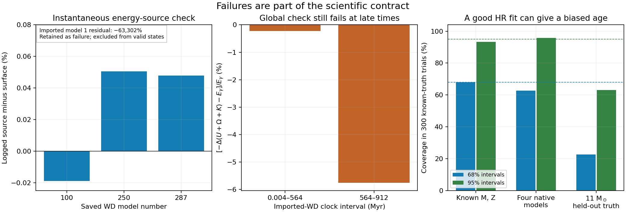
The local atlas tests are deliberately smaller. An independently computed eleven-solar-mass Solar history is withheld between ten and twelve. At matching absolute central hydrogen fraction, the largest HR discrepancy is about 0.31 of the stipulated synthetic observational scale, while the largest age discrepancy is about 1.8 percent.

The LMC holdout is more revealing. Linear-Z weights give an HR discrepancy as large as1.11 of that scale. Log-Z weights improve the largest HR discrepancy to about 0.44, yet the largest age discrepancy rises to about 9.2 percent. Better agreement in two surface coordinates has not validated the clock. This limited test examines two simple interpolation weights. The full MIST method and interpolated internal structures would each need their own validation.

Sources: Dotter (2016), MIST 0, arXiv:1601.05144v1, phase-aware track interpolation · Keszthelyi (2022), fixed reproduction package, Zenodo 7069766, CC BY 4.0

Compare instantaneous power with a finite energy change

Open MESA VI, arXiv:2208.03651v2, Section V and Equations 47–54. Follow the definitions of internal energy, composition terms and gravitational energy before interpreting an energy residual. Thermodynamic consistency of an equation of state and convergence of an evolutionary path are distinct from solving a chosen discrete equation accurately.

The saved white-dwarf example provides a direct test. Its first imported state gives an unphysical local source comparison and is excluded from the supported snapshots. In the three later states, integrating nuclear heat minus thermal neutrino losses plus gravothermal power matches surface luminosity within about 0.051 percent.

Perform another calculation: integrate stored internal energy, kinetic energy and self-gravity at two endpoints, then compare the change with photon energy radiated between them. The gravity integral used here is exact for cell-constant density and passes the analytic uniform-sphere test. This avoids using the same local luminosity equation as its own sole check.

For the late interval, the photon integral is about $5.19\times10^{46}\,\mathrm{erg}$ and the inferred decrease in those stored energies is about $4.89\times10^{46}\,\mathrm{erg}$ . The difference is about 5.75 percent. That larger discrepancy survives despite the good local source comparisons.

Sparse outputs do not identify a unique cause. A closer investigation would need consistent EOS and latent-energy definitions, the relevant source history, boundary terms and convergence tests. The current states show a cooling remnant and its structure, while the global energy disagreement limits precision cooling-age claims.

E=\int\left(u+\frac{v^2}{2}-\frac{Gm}{r}\right)dm,\qquad E_{\gamma}=\int L_{\mathrm{surface}}\,dt

Specific internal energy is

u

, radial speed is

v

, and

m

is enclosed mass. The spherical gravitational integral counts each shell’s interaction once. Additional physical sources and boundary terms must be included when making a complete energy balance.

Three panels retain the failed WD import, the late global energy mismatch and poor held-out stellar-age interval coverage. — Local WD source residuals are small in the later snapshots, yet the late finite-energy comparison differs by 5.75 percent. The right panel independently shows an age failure that the HR fit statistic does not reject.

Sources: Jermyn et al., MESA VI, arXiv:2208.03651v2, Section V energy consistency · Kumar and Townsley (2025), fixed white-dwarf cooling reproduction package, Zenodo 17765239, CC BY 4.0

Carry the unresolved questions into the next calculation

A useful next experiment changes one physical prescription in a matched family and separately refines its time and mass resolution. Keep initial abundances, starting model, network, atmosphere and stopping condition with every run. Save enough interior and energy information to repeat more than a surface-curve comparison.

For an observed star, add actual measurement covariances, distance and extinction information, abundance constraints and the model-selection assumptions. The current age exercise uses independent synthetic HR errors and a known truth. Its interval cannot absorb those missing observational or physical ingredients merely by becoming numerically precise.

When reading a new paper, ask three concrete questions: which physical term changed, which native calculation was withheld, and which independent quantity exposes a failure? Those questions connect the frontiers of mixing, winds and late burning to tests a reader can actually reproduce.

Sources: Paxton et al., MESA IV, arXiv:1710.08424v1, energy equations and convective boundaries · Jermyn et al., MESA VI, arXiv:2208.03651v2, Section V energy consistency · Dotter (2016), MIST 0, arXiv:1601.05144v1, phase-aware track interpolation