Recompute five fixed gas slices

Open the input before running the calculation

The file inputs/fixed-slices.json contains five snapshots. The first three use $q=0$ at frame 49, 64 and 128; their model times are minus 2.34375, 150 and 800 million years. The final two use $q=2.72$ and $q=4$ at frame 79, both at 302.34375 million years. They are our own synthetic results, not an observed galaxy catalogue.

Each slice carries 64 rows and 13 fields. The first six are Cartesian position and velocity in the galaxy rest frame, with the disk normal along $z$. Positions use kiloparsecs and velocities kiloparsecs per million years. The next fields retain work, dissipation, input energy, gas and birth mass, birth energy and birth angular momentum. Read fieldOrder before reshaping.

The common block gives initial radii, masses and fixed areas. The source-archive and full-record hashes identify where a slice came from; the public package contains selected slices with those source identities. Its fixed input SHA is e536102615f5fc2bfdda56b4374dc63fc0307229a0a248c6e84a7ab8ad2638ca.

Reading: Original fixed-slice and static-restoring-force materials

Run once in an ordinary Python environment

Unpack the ZIP into its own folder and install the declared dependencies in a virtual environment if needed. The calculation itself is offline. recompute.py calls the independent criterion.py, checks the supplied fixed reference and writes recomputed.json.

The script evaluates the slices, searches restoring-force maxima and calculates colour ratios from a small set of our band luminosities. It does not integrate new gas paths or rebuild the stellar spectrum convolution. Keeping that distinction visible tells you which part of the chain you have actually repeated.

The input numbers are written with full decimal roundtrip precision. Keep full roundtrip precision while calculating binding, then round the displayed values.

python recompute.py --out recomputed.json

Reading: Original fixed-slice and static-restoring-force materials

Make the disk and binding masks yourself

For each row, calculate cylindrical radius from the two in-plane coordinates. A row belongs to the disk only when radius is at most 16 kiloparsecs and the absolute height is at most 1 kiloparsec. Sum current gas mass over those rows, then divide by the 2000-million-year consumption time and convert to a yearly rate.

For binding, add half the squared speed to the external potential evaluated at the same position. The potential contains the declared bulge, halo and disk and tends to zero at infinity. Use all three velocity components. Positive energy gives the currently unbound mask; it is independent of the disk mask.

On the first $q=0$ slice you should recover an outside fraction 0.265625, a current unbound fraction zero, and a disk rate about 0.186096 solar masses per year. At frame 64, the outside fraction is still 0.265625 but the positive-energy fraction is 0.0625. This is a useful test against accidentally using the same mask twice.

Reading: Original fixed-slice and static-restoring-force materials

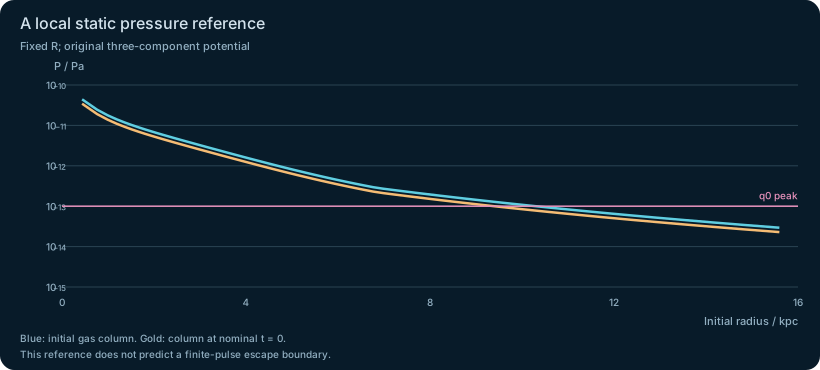
Rebuild the local static comparison

criterion.py differentiates the specified potential analytically to obtain the positive-height restoring acceleration. At each initial radius it samples a logarithmic height grid, locates every resolved local maximum bracket, and refines the candidates. The search extends to 10000 kiloparsecs; a total-mass inverse-square bound keeps the unsearched tail below the selected maximum.

It repeats the search on 256 and 512 grids. Preparation also compared 512 with 1024. These finite checks test whether changing the sampled brackets changes the numerical maximum. They are not a mathematical proof that an arbitrary, differently shaped potential has no unresolved peak.

Two pressure curves multiply the same acceleration by different columns: the initial mass divided by fixed area, and that column consumed to nominal closest approach, multiplied by the exponential factor for 500 million years. Actual sheets also move radially. The curves are explicitly fixed-radius quasi-static references, not a fitted stripping radius or a finite-pulse escape prediction.

Reading: Original fixed-slice and static-restoring-force materials · Köppen, Jáchym, Taylor & Palouš, Ram Pressure Stripping Made Easy, arXiv:1806.05887v1 (2018)

Check a force without trusting its own plot

The independent mathematical checks use two other routes. First, the vertical work integral of restoring acceleration must equal the potential difference between the midplane and a large height. Second, an isolated Plummer bulge has a known maximum, obtained by differentiating its simple analytic force. These tests check sign, units and the force–potential relation.

The preparation gave relative differences near 2.22 times ten to the minus 16 for both controls. Those tiny finite arithmetic residuals do not measure astrophysical uncertainty. The most consequential physical assumption remains the uniform centre-sampled wind applied even to the far tail.

Finally, compare disk and all-gas rates at matched times for $q=2.72$ and q4. The all-gas values should agree, while the weakly lifted gas changes the disk count. A result that instead claims global wind quenching has changed the prescribed consumption model.

Reading: Original fixed-slice and static-restoring-force materials

Keep a short calculation note

Record the input hash, units, model time, aperture definition, potential zero and numerical refinement. Keep the static reference separate from the actual trajectory result. If you change a column, potential or consumption time, save a new input and state exactly which comparison changed.

The population block is a second small exercise: it contains two input histories, three dust screens, four exact ages and five bands. The script recalculates $g-r$ from those band luminosities. Recomputing the original SSP convolution would additionally require the fixed native spectral input and its normalization conventions, discussed in the next chapter.

Reading: Original fixed-slice and static-restoring-force materials