Follow gain and loss through a layer
Let the path coordinate increase toward the observer. A short segment adds emissivity and removes a fraction of the intensity through absorption coefficient , measured in inverse metres. Its path integral is dimensionless optical depth.
Writing defines the source function. For a constant source, change variables to optical depth, multiply the transfer equation by its integrating factor and integrate. The result separates attenuated incident light from the layer’s own surviving emission.
For several layers, feed each output into the next layer in physical order. A photon emitted in the front layer crosses less intervening material than one emitted behind it. When temperatures differ, swapping the layers generally changes the spectrum.
Reading: Mangum & Shirley, How to Calculate Molecular Column Density, arXiv 1501.01703v4 (2017)
Kelvin on a brightness axis has a definition
LTE makes the source function equal to the Planck function. Radio data often express intensity in RJ-equivalent kelvin: a linear rescaling of intensity. That choice of units does not require replacing the Planck spectrum by its low-frequency approximation.
The function writes the full Planck intensity in those units. With a 2.725-kelvin incident background, the saved line excess follows the expression below. At 345 gigahertz, , so cold-gas calculations need the exponential factor.
For a complete numerical example, take gas at 20 kelvin. Then and the background term is . A line-centre optical depth of one gives of excess brightness. At very large optical depth the limit is . None of these brightness values equals the supplied 20-kelvin thermodynamic temperature.
Reading: Mangum & Shirley, How to Calculate Molecular Column Density, arXiv 1501.01703v4 (2017) · Sandbox Physics independent molecular-line science producer and reader package
Saturation changes width as well as height
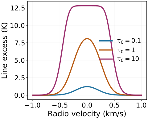
At small optical depth, expanding the exponential makes brightness nearly proportional to column. At large optical depth the centre is already close to the source function. More column mainly makes the wings opaque over a wider velocity interval.
The figure holds temperature and microscopic dispersion fixed. Its increasing optical depths produce a flatter, broader line even though the molecular velocity distribution is unchanged. A measured half-maximum width can therefore include a transfer effect.
A retained offline stress case increases an already thick column by a factor of ten. Its peak ratio is nearly one while its integrated-brightness ratio is about 1.178. That case lies outside the main Lab column range. It illustrates different saturation of peak and area, without turning either into a unique real-column estimate.
Reading: Sandbox Physics independent molecular-line science producer and reader package · Mangum & Shirley, How to Calculate Molecular Column Density, arXiv 1501.01703v4 (2017)
A static foreground can make two peaks
Place a cooler layer in front of a warmer emitting layer and give both zero mean velocity. The cool foreground absorbs most strongly near line centre. The centre can fall below the neighbouring wings, leaving two apparent peaks.
There are no oppositely moving parcels in this example. Assigning every double peak to two velocity components would miss a possible transfer explanation. Lines with different opacity or excitation conditions can help test that interpretation.
The interactive branch is isothermal rigid rotation. On each sightline, its temperature and mean recession speed are constant with depth. Every segment therefore shares the source function and normalized profile. Integrating density into a column and applying one slab solution is exactly equivalent to ordered transfer under those conditions.
Temperature gradients, inflow and a distinct cool foreground break that equivalence. The independent package keeps general sightline calculations for such offline examples. The fast branch is a mathematically justified special case; it does not solve arbitrary cloud excitation or dynamical evolution.
Reading: Sandbox Physics independent molecular-line science producer and reader package · Mangum & Shirley, How to Calculate Molecular Column Density, arXiv 1501.01703v4 (2017)