One frequency can contain two places
Imagine a sightline through a cloud. One parcel is nearby and another lies much farther along it. Both contain the same molecule and both recede at the same speed. Light from the same molecular transition reaches us at the same shifted frequency.
If the line is sufficiently transparent, light from the rear parcel passes through the front one. Their contributions add in one image pixel. Move the rear parcel farther back while preserving the stated angular extent, temperature, velocity and total molecular column, and the channel image can remain almost unchanged. The image has combined locations that were separate in space.
Only the component of motion toward or away from us supplies this first-order Doppler shift. A parcel can move rapidly across the sky without acquiring a large recession speed. A spectrum and a picture describe different parts of its motion.
Reading: Mangum & Shirley, How to Calculate Molecular Column Density, arXiv 1501.01703v4 (2017)
Molecules supply a recognizable frequency
A rotating molecule has particular allowed energy levels. A downward transition emits light at a characteristic frequency. Many molecules produce a narrow peak at that frequency, called a spectral line. Several useful rotational lines of CO lie at millimetre or submillimetre wavelengths, where radio telescopes can receive them.
Motion shifts the peak. Approaching gas is received at a slightly higher frequency; receding gas arrives at a lower one. A receiver divides the frequency range into small intervals. Each interval gives a channel image of the sky.
There is a width on both sides of this measurement. Molecules have a distribution of thermal velocities, and the receiver channel has a finite frequency width. A channel therefore admits a band of speeds with different weights. Narrower channels may reveal finer velocity structure, until physical line broadening becomes the limiting width.
Reading: Mangum & Shirley, How to Calculate Molecular Column Density, arXiv 1501.01703v4 (2017) · Leiden Atomic and Molecular Database, fixed CO data file
Rotation moves the bright region between channels
Tilt a cloud’s rotation axis away from the line of sight. One side moves toward us and the other recedes. The approaching side contributes to the higher-frequency channels; the receding side enters the lower-frequency ones. Scan through the line and the bright region moves across the cloud.
The receiver is selecting different parts of one snapshot. No searchlight has crossed the gas. A smooth distribution of molecules can make distinct patches in a narrow channel because different locations have different velocities.
Another useful view takes a line across the image and stacks the full spectrum at each position. This produces a position–velocity diagram. One axis is sky position and the other is velocity. Rotation can make a tilted bright band. The vertical coordinate of that diagram still describes motion.
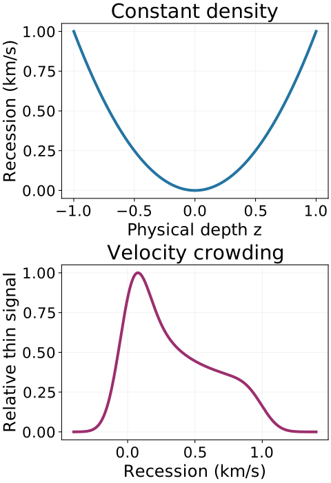
Reading: Lazarian & Pogosyan, Velocity Modification of HI Power Spectrum, astro-ph/9901241v2 (2000) · Sandbox Physics independent molecular-line science producer and reader package
Try sorting three parcels
Suppose one parcel approaches at six hundred metres per second. Two others recede at two hundred metres per second, one behind the other. A channel near the latter recession speed mainly selects those two parcels. Move to the approaching speed and the first parcel becomes bright.
This separation works cleanly when the physical line widths are small compared with the gap between the two velocity groups. Broad thermal or microscopic velocity distributions can make the peaks overlap. Temperature and absorption can also change how strongly different layers contribute.
For a real cloud, begin by following a patch through adjacent channels. Then inspect its full spectrum and ask whether the patch survives when the channels are integrated. These connected views help turn an attractive image into a more specific question about gas motion.
Reading: Mangum & Shirley, How to Calculate Molecular Column Density, arXiv 1501.01703v4 (2017) · Sandbox Physics independent molecular-line science producer and reader package