Slide a predicted chirp across the measured strain and look for the time when their crests line up. At the right shift, a whole run of small oscillations adds in the same direction. Random bumps in the detector usually give up their gains a few cycles later. That is the idea of a matched filter.
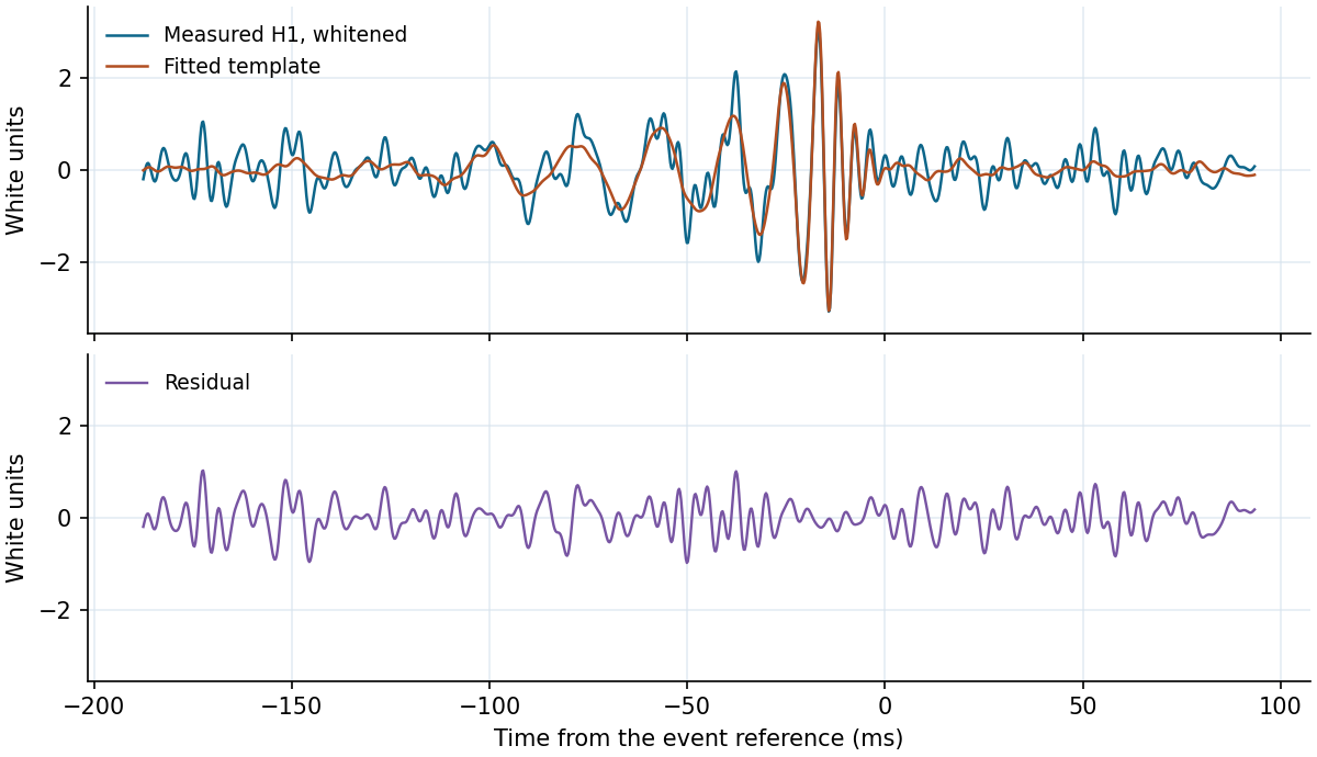
Whitened Hanford strain, the fixed-family fit and the remaining trace.
A wave with a changing pace
On a raw plot of the Hanford strain, slow motion and narrow noise lines can look larger than the event. The detector is still measuring a very small fraction by which the two arms change their relative length. The strain trace carries that measurement and the noise together.
A compact binary chirps faster as its orbit shrinks. Imagine laying a thin tracing of that pattern over the data. If it sits a few cycles early, a crest on the tracing may be over a trough in the data. Slide it to the right place and many of the same crests arrive together. The resulting score gets its strength from their agreement over time. GWOSC worked event tutorial
Listen where the detector is quiet
An instrument can be quiet at some frequencies and noisy at others. The filter gives quieter frequencies more weight, judged from nearby data away from the event. After that weighting the part of the trace with GW150914 is easier to see, though individual noise peaks are still there. LIGO–Virgo detector noise guide, §4
Use the Hanford view in the analysis. Move the vertical arrival marker a few tens of milliseconds. The fitted chirp still has the same shape, but its peaks slip off the observed ones and the score falls. Move back to the peak. In the residual, what remains after subtracting the fitted template, the run of coherent crests is weaker. Then switch to Livingston and look for its own peak. The two sites pick up similar patterns at slightly different times.