Recalculate a bar orbit from saved states

Open the small package before running it

The scientific ZIP contains only own Python producers, numerical inputs, provenance and explanatory text. Its manifest identifies every member except itself. The replay checks that inventory before calculation and refuses a changed byte or an existing output directory.

The field is $\Phi=\ln R+Af(R)\cos[2(\phi-\Omega_pt)]$, with $A=0.01$, $\Omega_p=1$ and $R_b=0.5$. Population coordinates are inertial. Periodic-parent coordinates rotate with the bar. Energy and angular momentum are specific quantities; no physical Milky Way length or mass has been fitted.

To compare with the interactive experiment, select either parent preset, which uses this same field. Its main default has a stronger amplitude of 0.04 and is a different release.

python3 -W error replay.py --output /absolute/new/empty/run

Reading: Sandbox Physics independent galactic-bar scientific reader v1 · Dehnen (1999v1/2000), The Effect of the Outer Lindblad Resonance of the Galactic Bar on the Local Stellar Velocity Distribution

Follow the six fresh commands

The first producer integrates 256 tracers at 5120 and 10240 steps, then saves the fine result. The second compares ten original test states with a polar-force DOP853 integrator, measures an exact circle and small epicycle, and integrates prescribed amplitude growth. The next two commands solve the inner and outer parent roots and complete their periods.

The fifth command reads the completed files and calculates diagnostics. The sixth draws the figures from those same saved arrays. None of the numerical results is shipped inside the package. Every command runs serially with a 120-second ceiling.

On the author's first cold run, the six commands took $23.37\,\mathrm{s}$ including first-time plotting/font work and wrote about $1.90\,\mathrm{MB}$. That is a local timing, not a promise for every computer. The receipts report each command separately.

Reading: Sandbox Physics independent galactic-bar scientific reader v1

Read the saved angular momentum and torque together

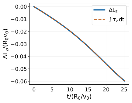
Open population/population-record.npz. Its arrays contain times, four-component inertial states, equal sampling weights and the fine-step torque integral. For each saved state calculate $L_z=xv_y-yv_x$. Subtract the initial value and compare with the saved time integral of torque.

The plotted selected tracer has final $\Delta L_z\simeq-0.0596448$. Its axisymmetric reference guiding radius falls by the same numerical amount because $v_0=1$. This does not identify its instantaneous radius or establish a permanent migration endpoint.

The saved torque discrepancy is around $4.7\times10^{-14}$. KDK kicks and the matched torque quadrature share a discrete angular-momentum identity, so this near-roundoff agreement is an internal consistency check. The independent ten-state trajectory comparison gives a much larger and more relevant error, about $2.44\times10^{-5}$ in the registered scaled norm.

Reading: Sandbox Physics independent galactic-bar scientific reader v1

Inspect errors over the whole history

For the entire population the largest middle/fine difference, divided by three, is $2.53\times10^{-5}$, below the registered $2\times10^{-4}$ threshold. Its minimum radius over every fine drift is about $0.7814$. Neither statement is inferred from 257 saved frames alone.

The six newly shot parents return within about $1.3\times10^{-14}$ in the reference scaled norm. Separate KDK integrations at three steps test complete trajectories against those references. The tiny shooting residual should not be confused with the larger discretisation error of a different integrator.

The population statistic $Q_2$ averages the complex double azimuth with equal weights. Its amplitude describes this sample's angular anisotropy. It does not weight surface area, mass, stellar ages or luminosity, and it cannot serve as a galaxy brightness map.

Reading: Sandbox Physics independent galactic-bar scientific reader v1

Keep the examples that fail

The wide bracket at starting radius 1.45 has negative return velocities at both endpoints. Replay reports the actual residuals and keeps the failed bracket. The six successful parents use their separately declared narrow brackets.

The fast warm release $A=0.04,\Omega_p=1.4,\sigma_R=0.08$ crosses the admitted radius $R=0.5$. This reader stops at its first invalid drift and retains that state. It does not complete a scientifically admitted trajectory by ignoring the crossing.

The growth example retains a failed constant-Jacobi hypothesis, then tests the correct amplitude-work relation. These expected failures remain scientifically failed even when the wrapper successfully reproduces them.

Reading: Sandbox Physics independent galactic-bar scientific reader v1

Carry the method to a new calculation

Write down the frame, units, initial sampling and complete time history before interpreting a curve. Use a quantity's actual sampling weights. Compare full trajectories with an independent solver or analytic limit as well as checking invariants.

Change one physical condition only after registering its error and domain tests. If a new orbit crosses the excluded inner branch, preserve the failed input. If a perturbation grows or fades, include its explicit work before judging conservation. A saved endpoint is a point in that history, not a substitute for it.

Reading: Sandbox Physics independent galactic-bar scientific reader v1 · Sellwood & Binney (2002), Radial mixing in galactic discs, astro-ph/0203510v2