Recalculate a published benchmark and test a public jet spectrum

Open Cowan and collaborators’ arXiv:1007.1727v3 at Section 5.1.1 and Figure 7. You will recalculate its known-background counting example, then use a frozen CMS jet table to test the extrapolation of a simple empirical shape. The first exercise reproduces a specified published statistical calculation. The second asks a deliberately narrower question than the CMS QCD analysis: how far can a low-order shape describe the published spectrum?

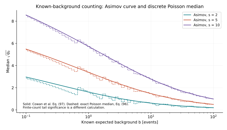
Figure 7 compares a smooth approximation with discrete counts

The horizontal axis is the expected background count, scanned from 0.1 to 100 in our saved calculation. The paper compares signal yields of two, five and ten. The vertical quantity is the median discovery-significance approximation for a known background. This example has one counting region, no nuisance parameters and a fixed signal hypothesis.

Equation (96) gives the square root of the one-sided likelihood-ratio statistic for an observed count. Equation (97) replaces the count by its expected signal-plus-background value, called the Asimov value. For positive signal yield $s$ and known background $b$, it gives

A logarithm expansion recovers the familiar signal divided by the square root of background only when the signal is small compared with the background. The signal-to-background ratio therefore matters as well as the total count.

Recalculate the staircase without a random generator

Find the smallest integer whose Poisson cumulative probability at mean $s+b$ reaches one half. This is a defined discrete median count. Put that count into Equation (96). The resulting staircase is the exact Poisson median of the statistic’s square root; converting it to an exact finite-sample Gaussian-equivalent tail significance would require a separate null-tail calculation.

For signal two and background 0.1, the median count is two. The Asimov expression gives about 2.964, and the discrete-median square root gives about 2.861. Their difference comes from count discreteness. The saved calculation covers 183 signal-background points. An independent numerical optimization of the Poisson likelihood agrees with the closed-form statistic to a maximum absolute difference of about two parts in ten trillion.

Run the repository’s cowan-counting-benchmark.py script to regenerate the table. The downloadable JSON states the paper version, equations, signal yields and background range. The accompanying plot recalculates that bounded slice of Figure 7. The paper’s nuisance-parameter examples require their own models and calibration.

Freeze one measured jet spectrum before fitting it

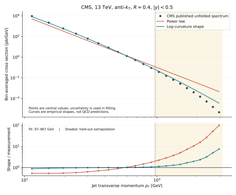
The data product is HEPData record 115022, version two, table ak4_xsec_ybin1, with its table-five correlation matrix. It contains 22 published unfolded bins from 97 to 3103 GeV for anti-kT radius 0.4 and absolute rapidity below 0.5, from CMS proton collisions at 13 TeV. The table uses $\mathrm{pb/GeV}$, with $1\ \mathrm{pb}=10^{-40}\ \mathrm{m}^2$. These are published particle-level spectrum values, not raw collision events and not newly unfolded records.

The provenance download fixes the table DOIs, filenames, byte counts, SHA-256 hashes and the CC0 data licence. The paper is arXiv:2111.10431v3, with the December 2022 addendum linked separately. The addendum revises the strong-coupling interpretation; the old abstract’s fit value should not be repeated as the corrected result. This exercise extracts no strong coupling or Wilson coefficient.

Average the predicted curve over each published bin

A steeply falling curve can differ appreciably between a bin centre and its bin average. Fit the average over the exact published edges. Our empirical model uses $u=\ln(p_T/(500\ \mathrm{GeV}))$ and

Setting curvature $k$ to zero gives a power law. Allowing curvature lets its logarithmic slope change. Neither expression contains the parton distributions, perturbative hard coefficients or nonperturbative corrections needed for a QCD prediction.

The fit uses the first twelve bins, through 967 GeV. The ten higher bins are held out of parameter estimation. Shared systematics correlate the held-out and fitted bins; the extrapolation retains these dependencies.

Keep signed systematic shifts and unfolding correlations

The table-five matrix describes correlations of a combined statistical and binwise-uncorrelated-systematic component after unfolding. Named signed systematic shifts from the spectrum table supply additional correlated components. The calculation builds their outer products within this one rapidity slice, then uses a covariance linearized in the logarithm of the cross section for generalized least squares.

This approximation is frozen as part of the method. It uses no cross-rapidity or theory covariance and gives no predictive p-value or fitted-parameter uncertainty. The paper’s Figure 3 discusses correlations for the other jet radius. This exercise uses the corresponding AK4 table and keeps its source distinct from that figure.

Both simple shapes fail the precision test

The power-law training statistic is about 5673 for ten degrees of freedom. Curvature reduces it to about 164 for nine degrees of freedom. Both are already inadequate at the quoted experimental precision. In the held-out range the root mean square of prediction-to-data fractional residuals is about 36.8 for the power law and 2.60 for the curved shape. These ratios are dimensionless; 2.60 means 260 percent, not 2.60 percent.

The curved extrapolation is closer, yet still far from a precision description. The failure supplies no evidence for a new particle. It shows that choosing a convenient background family can leave a large residual even with real published data. The analytic power-law bin integral agrees with independent quadrature to about seven parts in ten quadrillion, which checks integration accuracy without making the model physically adequate.

Compare a published QCD-model correction envelope

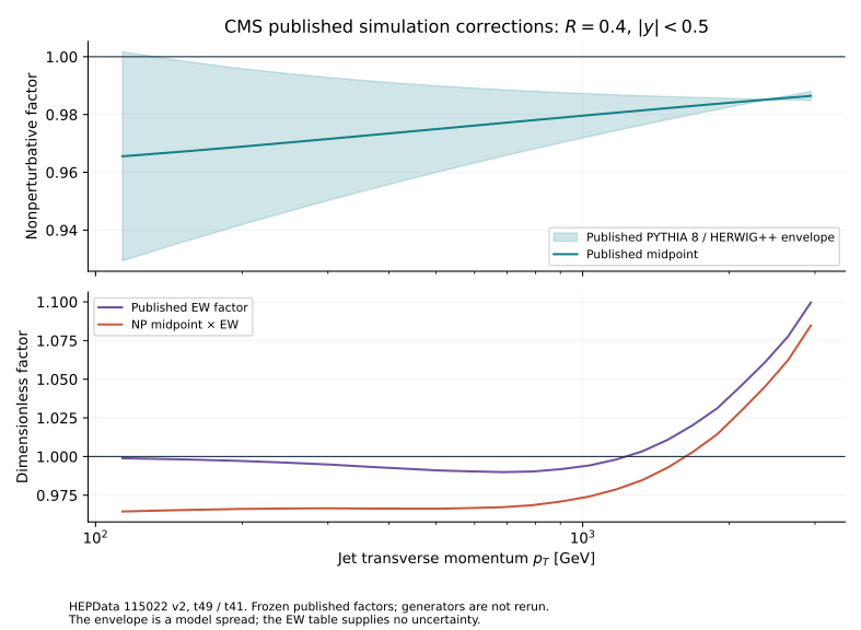
The same frozen release supplies nonperturbative correction factors in table 49 and electroweak factors in table 41. The paper defines the nonperturbative factor as a simulated cross-section ratio: shower plus multiparton interactions and hadronization, divided by shower alone. A smooth envelope from PYTHIA 8 CP1 and HERWIG++ EE5C estimates model dependence. The table gives a central midpoint and half-width; its endpoints are not individually labelled by generator.

For the first momentum bin the nonperturbative factor is 0.96555 with envelope half-width 0.036159. Multiplying its central value by the separate electroweak factor 0.99888 gives 0.964469. Across the frozen bins the combined central factor reaches 1.08471 in the highest bin. These dimensionless model corrections are separate from the measured cross-section values. The downloadable report preserves both columns, and the electroweak table’s missing uncertainty should not be read as zero theory error.

The accompanying correction plot recalculates a bounded central-rapidity slice associated with Section 4.3, Equation (4) and Figure 5a. It uses published model factors; no shower, hadronization generator or fixed-order prediction is rerun. This supplies a concrete comparison of published model dependence alongside the empirical shape diagnostic.

A repeatable reading task

Run public-spectrum-benchmark.py and compare the saved training split, fitted coefficients and residual arrays. Then move the split only in a separately labelled study. Ask whether the conclusion changes because of the model, the fitted momentum range or the uncertainty assumptions. Keep the frozen table unchanged.

For the jet paper, return to anti-kT Equation (1) and Figure 1. Recalculate an isolated hard particle’s soft capture radius using the distance comparison from Chapter 4. That tests the stated analytic limit. Reproducing the whole Figure 1 would additionally require its generator event, ghost definition and clustering-area setup.

Questions to answer before reusing a result

Question 1. Why does matching a curve visually on logarithmic axes give weak evidence of a good fit?

Answer. A log plot compresses large relative differences across many orders of magnitude. Compare bin averages and correlated residuals with their stated uncertainties; the training statistics here expose a failure that a thumbnail can conceal.

Question 2. Can this spectrum be fed directly into the Poisson-count likelihood of Chapter 6?

Answer. No. It is an unfolded cross section with correlations and systematic components, not independent integer counts. A statistical model must match that published data product, or use the underlying event-level likelihood when available.

Question 3. What would a genuine EFT interpretation add?

Answer. A defined operator basis and order, QCD and parton-distribution predictions, detector or published-result likelihood, correlated experimental and theoretical uncertainties, and an energy-validity treatment. The CMS paper performs a much larger analysis; this bounded shape exercise is preparation for reading it.

Inspect the calculated figures

• Counting benchmark values and definitions
• Spectrum fit, covariance method and residual arrays
• Original CMS spectrum table JSON
• Original CMS correlation table JSON
• Published QCD-model correction comparison
• Original nonperturbative-correction table JSON
• Original electroweak-correction table JSON
• Provenance, hashes and data licence
• Source code: counting benchmark
• Source code: public-spectrum shape check
• Source code: published model-correction envelope
• CMS December 2022 addendum