Reading a Wilson–Fisher flow diagram

Different microscopic models can approach the same long-distance behavior when coarse graining carries their parameters toward the same fixed point. The Wilson–Fisher calculation makes this idea quantitative for a real scalar field in dimensions slightly below four. It also shows why reaching a critical point usually requires tuning a parameter: one direction of the flow leads away from it.

This chapter uses keeping low-energy physics and finite-size scaling. You should know what an effective action, a correlation length and a critical exponent mean. We will introduce a beta function as the rate at which a parameter changes with scale, then use a linear approximation to find which perturbations grow.

Let the scale change the parameters

Start with a real scalar field with sign symmetry: changing the sign of every field value leaves its probability unchanged. Its Euclidean action includes a gradient term, a mass term and a positive quartic interaction. Integrating a momentum shell changes their coefficients. Rescaling coordinates and the field then restores a common cutoff and gradient normalization, so that we can compare successive theories.

Let $\zeta$ be the factor by which the observation length grows, and write $s=\log\zeta$. Increasing $s$ moves toward longer distances, the infrared direction. We use dimensionless mass $r=\mu^2/\Lambda^2$ and coupling $u=9\widetilde g/(2\pi^2)$, where $\Lambda$ is the restored momentum cutoff and $\widetilde g$ is the dimensionless quartic coefficient in Tong's convention $\widetilde g\phi^4$. The cutoff is set to one in numerical calculations.

The dimension is written $d=4-\epsilon$. Here $\epsilon$ is a small positive expansion parameter. A noninteger dimension enters the analytic formulas; it does not describe the geometry of the one-dimensional ring in the preceding experiment.

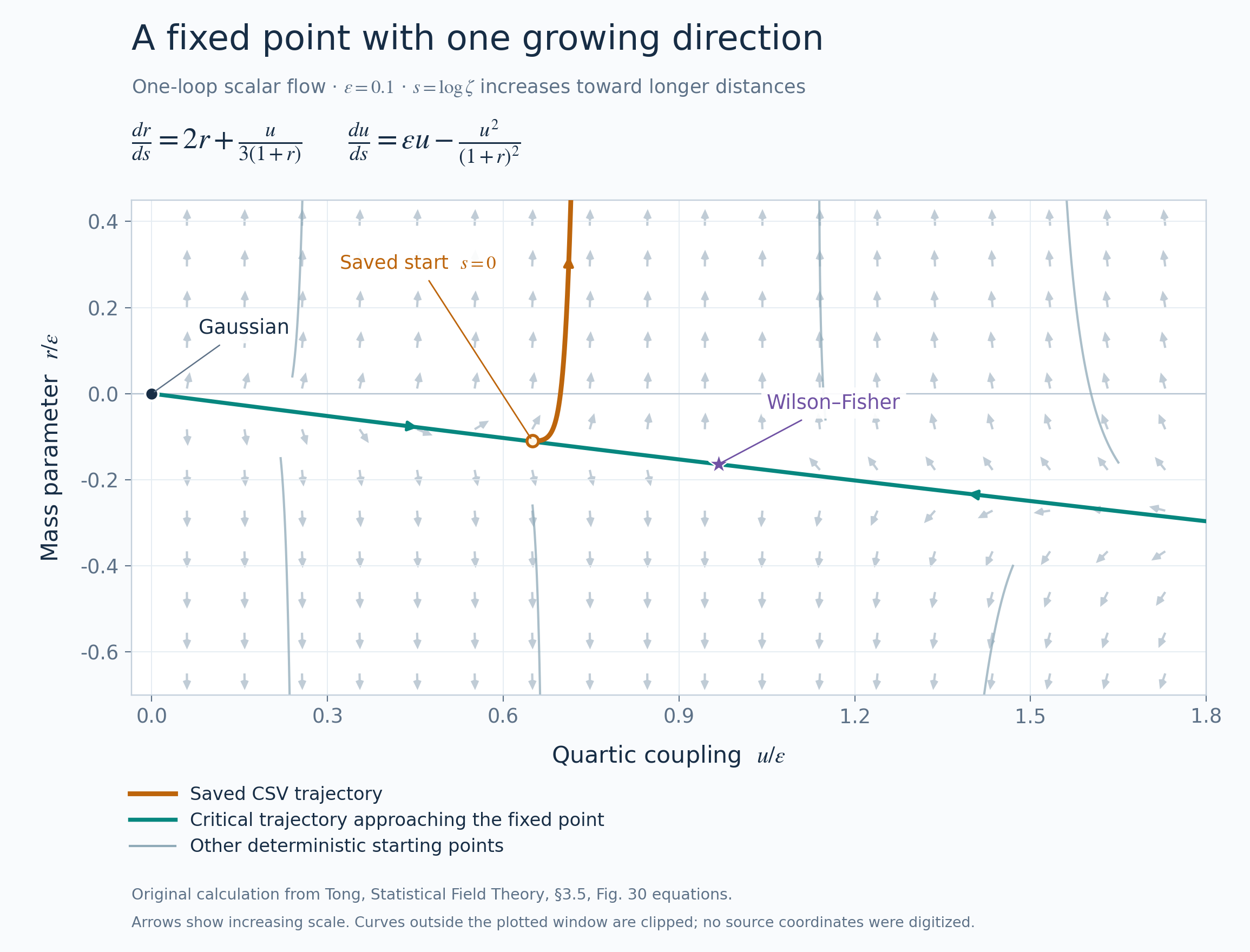
Even before doing an interaction calculation, rescaling tells us something. Keeping the gradient term normalized makes a mass term grow as $\zeta^2$, while the quartic term grows as $\zeta^{4-d}$. Thus their initial rates contain $2r$ and $\epsilon u$. The loop correction expresses the effect of integrating over the short-wavelength field. At one loop, Tong's section 3.5, printed page 90, gives the normalized equations

The right sides are beta functions. They specify an arrow at each point in parameter space. A trajectory follows those arrows as the observation scale increases.

Find a point that the flow leaves unchanged

A fixed point makes both beta functions vanish. The origin $r=u=0$ is the Gaussian fixed point. To find another, suppose $u$ is positive. The second equation then gives

Substituting into the first equation leaves $2r_*+\epsilon(1+r_*)/3=0$. Solving gives the nonzero fixed point of the displayed, truncated equations:

At first order, these become $r_*=-\epsilon/6+O(\epsilon^2)$ and $u_*=\epsilon+O(\epsilon^2)$. A small $\epsilon$ puts the fixed point at a small coupling, where the perturbative calculation can be controlled.

For a worked example, take $\epsilon=0.1$. The truncated equations give $r_*\approx-0.0163934$ and $u_*\approx0.0967482$. Substitute these values into both beta functions: each vanishes to numerical rounding. Their algebraic expressions contain powers of $\epsilon$ beyond first order because we solved the truncated equations exactly. Those powers originate from exact algebra within a one-loop truncation.

One disturbance grows and another shrinks

Finding a stationary point does not tell us whether nearby trajectories approach it. Write $r=r_*+\delta r$ and $u=u_*+\delta u$. For small deviations, expand the beta functions to first order in the deviations. The matrix of derivatives tells us the local flow.

At the nonzero fixed point, its entries are

The lower-left entry starts at second order in $\epsilon$. To first order, the two eigenvalues are $y_t=2-\epsilon/3$ and $y_u=-\epsilon$. An eigenvector identifies a particular combination of the mass and coupling disturbances. Along it, a disturbance changes as $e^{ys}$.

A positive $y$ makes a disturbance grow; that direction is called relevant. A negative $y$ makes it shrink; that direction is irrelevant. Near the Wilson–Fisher point there is one of each. The thermal direction is a mixture of the original parameters, not simply an arbitrary horizontal or vertical line on the plot.

This explains both tuning and universality. Tuning the relevant disturbance toward zero lets a trajectory spend more scales close to the fixed point. Differences along the irrelevant direction shrink during that journey. Many different short-distance starting points can therefore share the same long-distance exponents.

Turn the flow into an exponent

Let $t$ be a dimensionless distance from criticality along the relevant thermal direction. After a scale change $\zeta$, it becomes $\zeta^{y_t}t$. Stop coarse graining when this reaches order one. Solving $\zeta^{y_t}|t|\sim1$ gives $\zeta\sim|t|^{-1/y_t}$. The correlation length grows by this same scale factor, so

The last expression expands the reciprocal consistently through first order. At $\epsilon=0.1$, it gives $\nu\approx0.508333$ at that order.

Susceptibility adds the connected correlation over space. If the critical correlation falls as distance to the power $-(d-2+\eta)$ and is cut off at distance $\xi$, this spatial integral grows as $\xi^{2-\eta}$. Thus $\gamma=\nu(2-\eta)$. The anomalous exponent $\eta$ begins at second order for this scalar expansion, giving

At $\epsilon=0.1$, the first-order value is $1.016667$. The coefficient $1/6$ is also the Ising-like susceptibility coefficient stated in the official abstract of Wilson and Fisher's 1972 paper, Critical Exponents in 3.99 Dimensions.

Read a reconstructed flow diagram

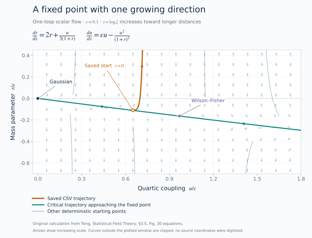
Open the lower flow panel of coarse graining and renormalization flow. It numerically reconstructs the equations behind Tong's Figure 30, printed page 91. The source figure is schematic. The plotted curves are new integrations of its equations, not digitized source coordinates or experimental data.

At the default $\epsilon=0.1$, the gold starting point is $r=-0.011$, $u=0.065$. Drag that point. Predict which changes make the trajectory leave the fixed point's neighborhood more quickly, then compare its direction with the nearby arrows. The axes divide each parameter by $\epsilon$ so that the small-coupling structure remains visible when the expansion parameter changes.

Export the flow CSV. It records the normalization, expansion parameter, step and scale coordinates. The reference trajectory uses fourth-order Runge–Kutta with step $0.025$. Halving that step changes its mass coordinate at $s=1$ by about $8.85\times10^{-11}$. This checks numerical integration accuracy. The omitted higher-loop corrections remain a different source of error.

Tong's equations and Figure 30 were checked against this calculation. Wilson and Fisher's 1972 published abstract supplies the historical first-order exponent check; its full PDF required authorization. The saved source report records that reading scope and the numerical parameters.

A discrete calculation from the published paper

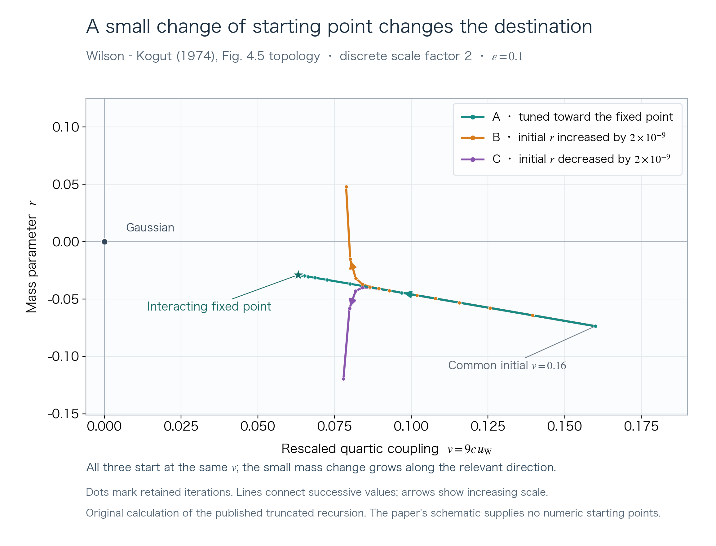
Wilson and Kogut's published 1974 review supplies a second calculation with a finite coarse-graining step. In section 4, Figure 4.5, printed page 108, one tuned sequence approaches a fixed point while two nearby sequences turn away. We can reconstruct that pattern directly from their equations (4.26)–(4.27), printed page 106.

Each step integrates the shell between momentum cutoffs $1/2$ and $1$, then restores the cutoff to one. The observation length doubles. To distinguish the paper's coupling $u_{\mathrm W}$ from the earlier convention, define $v=9c u_{\mathrm W}$, where $c=4\int_{1/2<|p|<1}d^d p/(2\pi)^d$ is a positive shell-volume factor. The paper's truncated recursion becomes

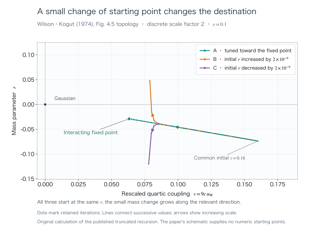
The figure below uses $\epsilon=0.1$. The tuned initial values are $v_0=0.16$ and $r_0\approx-0.0736025858656632$. Substituting once gives $r_1\approx-0.0641276051060$ and $v_1\approx0.139513337325$. Repeated substitution approaches the truncated map's fixed point, $r_*\approx-0.0289028753$, $v_*\approx0.0631518729$. The source figure supplies no numerical starting points; these values define our new calculation of its critical and escaping trajectories.

Keep $v_0$ fixed and predict what happens if $r_0$ increases by $2\times10^{-9}$. Compare the orange sequence B with the green sequence A, then try the same decrease, shown in purple as C. Both changed sequences first move toward the neighborhood of the fixed point. By iteration 13 they have turned away on opposite sides. A continues approaching through the 190 retained steps. The linked source record preserves every point and the full initial precision.

Why does such a small change matter? Linearizing this discrete map gives multipliers about $0.923935$ and $3.91500$: one disturbance shrinks per step, the other grows. A multiplier acts once for each doubling of length. Thus $y_t=\log\lambda_t/\log2$ and $\nu=\log2/\log\lambda_t$. Expanding consistently gives the paper's $\nu=1/2+\epsilon/12+O(\epsilon^2)$, in agreement with the continuous calculation. The exact algebraic value from this truncated map, about $0.507869$ at $\epsilon=0.1$, includes terms beyond that first-order expansion.

The tuned sequence also amplifies rounding errors. Its CSV therefore retains 180-digit arithmetic; replaying a rounded starting point in ordinary precision can eventually depart from A. The numerical checks compare higher precision and a nearer critical endpoint. Physical accuracy remains limited by the terms omitted from the source recursion. This published-paper reproduction covers Figure 4.5's topology and its first-order exponent, with explicit parameters and retained iterates.

Where universality can change

Symmetry, dimension and interaction range help decide which fixed points a theory can reach. A scalar with sign symmetry and short-range interactions has a different set of possible flows from a field with a continuous vector symmetry. Long-range couplings can change which terms remain important. A first-order transition can also prevent the approach to the critical fixed point considered here.

The small-$\epsilon$ calculation provides a controlled neighborhood below four dimensions. Setting $\epsilon=1$ does not by itself provide a precise three-dimensional exponent. Numerical finite-size scaling and other methods must address their own approximation errors. The conformal bootstrap review by Poland, Rychkov and Vichi describes another approach: consistency conditions on correlation functions at a conformal fixed point constrain the possible theory. It is an onward reading route; no bootstrap computation is performed in this experiment.

Exercises

• Set the coupling to zero in the flow equations. Solve for the mass parameter as a function of $s$ and explain the Gaussian thermal eigenvalue.
• Compute the first-order $\nu$ and $\gamma$ at $\epsilon=0.06$. Which digits would you retain when describing them as physical predictions?
• Two lattice actions have different bending terms but the same symmetry and short-range interactions. Under what additional condition could they share critical exponents? Why is their similarity alone insufficient?
• A very accurate numerical integration at $\epsilon=1$ returns many decimal places for an exponent from a one-loop formula. Identify two different uncertainties and explain which the small integration step addresses.