Calculate migration times and reconstruct Kepler-223 angles

Calculate a local migration-time map

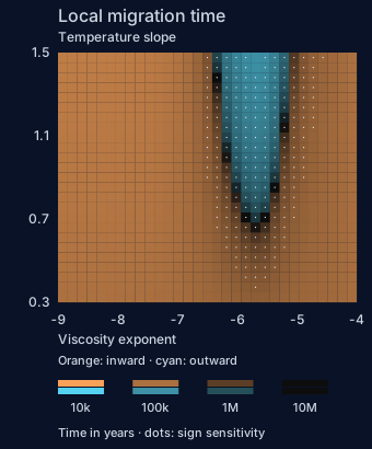
Fix a four-Earth-mass circular planet at one AU, height ratio 0.055 and density scale 0.0001. The public script evaluates 25 temperature slopes from 0.3 to 1.5 and 31 logarithmic viscosities from one billionth to one ten-thousandth in model units. Each of the 775 cells stores both torque contributions, signed drift and local migration time.

The frozen grid has 678 inward and 97 outward cells. Dots flag 222 cells whose net sign can reverse under a chosen twenty-percent perturbation envelope on the individual torque contributions. This is a deterministic sensitivity test, not a confidence interval or a calibrated error distribution. The physical law and units are the same as the preceding chapters.

Near cancellation the local time grows very large and diverges at an exact torque zero. It is radius divided by the current drift rate, not an integrated arrival time. Changing radius, disk evolution or a dynamical torque can change the subsequent route. The static zero is a useful place to test additional physics.

\tau_{\rm local}=\frac{a}{|\dot a|},\qquad \nu=10^x\,\mathrm{AU}^2/t_0

The map horizontal coordinate is the viscosity exponent; color shows direction and the logarithm of local time. Exact zero drift is stored as an infinite-time null with an explicit meaning.

            python3 migration-timescale-map.py --output my-map.json --figure my-map.svg

Reading: Paardekooper · Cresswell & Nelson

Know exactly which measurements you have

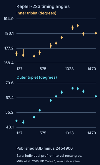
The input contains all forty-four quarterly transit-time shifts in Mills et al., arXiv:1612.07376v1, Extended Data Table 1: eleven bins for each of planets b, c, d and e. These are fitted timing measurements from real Kepler photometry, not synthetic transit times, individual transits or posterior draws.

The frozen author manuscript is 4,229,509 bytes with SHA-256 ee22071732db64c776a333b99e3e487c7e4ec3ca246cb52c1a1ed5c00f2b8115. The table is PDF page thirty. We redistribute factual numerical measurements with citation and our own scripts, not the paper’s text, figures or code. The table says BJD minus 2454900 without explicitly naming a dynamical time scale; no UTC or TDB conversion is invented.

Reading: Mills et al. · Izidoro et al.

Keep the table’s linear ephemerides

Each measured shift is relative to a particular reference ephemeris. Using the fitted dynamical periods from another table would change the diagnostic. The input metadata therefore stores the exact four reference periods and zero-transit epochs from Extended Data Table 1.

Quarter bins are matched by chronological index, but each planet’s mean observing time differs. Choose the arithmetic mean of those four actual times for a common diagnostic time. Within each bin hold the measured timing shift constant; then repeat the calculation at the earliest and latest planet mean time to measure alignment sensitivity.

Planet	Reference period (days)	Zero transit (published BJD offset)
b	7.3840154	70.49489
c	9.8487130	71.37624
d	14.7883997	109.76775
e	19.7213435	68.10686

Reading: Mills et al. · REBOUND 5.2.2 and IAS15

Convert a late transit into orbital phase

For an edge-on nearly circular orbit, a transit is assigned a quarter turn of mean longitude under the paper’s convention. If a transit occurs late, its phase at the reference time is behind the unshifted prediction. That fixes the minus sign of the timing shift.

Use the near-circular mean-longitude approximation to form two adjacent-triplet Laplace angles and their four-body combination. The third is algebraically dependent on the first two; it is not a third independent detection.

\lambda_i(t)\simeq\frac\pi2+\frac{2\pi}{P_i}(t-T_{0,i}-\delta T_i)

This approximation is not the full eccentric photodynamical transformation.

\phi_1=-\lambda_b+2\lambda_c-\lambda_d,\qquad\phi_2=\lambda_c-3\lambda_d+2\lambda_e

Integer coefficients cancel a common longitude zero point.

\phi_3=-3\phi_1+2\phi_2=3\lambda_b-4\lambda_c-3\lambda_d+4\lambda_e

Compute this combination directly from the original timing coefficients, preserving the reuse of the same measurements.

Reading: Mills et al. · Izidoro et al.

Run the public files in an empty folder

Download the listed scripts, CSV, source metadata and two synthetic reference records. The basic calculation uses Python’s standard library only and does not import this website, a private repository or a Lab Engine. It prints the torque grid, measured-angle ranges and an independent short RK4 check of a synthetic replay.

The checksum manifest verifies the frozen scientific inputs and scripts. Hashes certify exact bytes; numerical outputs are compared with tolerances because Python versions can differ in their last floating-point digits. The script does not claim to regenerate the entire long IAS15 history.

            python3 reproduce-migration.py --directory . --output my-results.json
python3 analyze-kepler223.py --directory . --output my-angles.json

Reading: Mills et al. · REBOUND 5.2.2 and IAS15

Read the actual output and its sensitivity

The reconstructed angles stay within the ranges below over the observed eleven bins. Changing the common time from the earliest to latest planet mean time changes the diagnostic by less than one degree in these data. This small alignment sensitivity does not remove the near-circular approximation or the finite observing window.

Each published timing interval is asymmetric and given as a signed offset from its best value at stated changes in chi-square. The script propagates a rectangle made from the four individual intervals by taking extrema of the linear combination. That envelope is neither a joint confidence interval nor a credible interval. It assumes no fabricated independence and supplies no posterior probability.

Combination	Observed-window range (degrees)	Largest quarter-time sensitivity (degrees)
Inner triplet	172.440–190.844	0.216
Outer triplet	47.075–75.434	0.786
Four-body combination	294.286–316.566	0.924

Reading: Mills et al. · Izidoro et al.

Separate two reproductions

The timing calculation reproduces a limited diagnostic from real measured data. Separately, the synthetic torque grid verifies the Lab’s local prescription, and an independently authored fourth-order Runge–Kutta integration checks an eight-orbit clip against IAS15. With maximum code-time steps 0.04, 0.02 and 0.01, the largest Cartesian differences shrink from 0.00001096 to 0.0000000208 in the adopted length or velocity units.

For a full synthetic rerun, download the optional generator, orbit and disk modules, packer and C force source. Install pinned REBOUND 5.2.2 in a separate environment; the generator also works with a Python force callback. Compiling the optional force source speeds a long rerun. The website distributes no compiled executable. Record actual integrator, parameters, duration, phase cadence and stop reason when making a new comparison.

Reading: REBOUND 5.2.2 and IAS15 · Paardekooper

Say what this has not established

A short bounded angle arc does not by itself prove long-term resonant stability. The original paper’s interpretation also uses interacting-orbit fits and stability calculations. Eccentricity, projection, priors and the covariance of the fitted parameters matter; the quarterly table cannot recreate all of them.

Likewise, a synthetic two-planet disk model does not infer the birth locations or disk parameters of this real four-planet chain. Testing that history requires a forward model tied to the observations and an explicit comparison of competing histories.

Reading: Mills et al. · Izidoro et al.

Download and run without this website

Synthetic local migration-time map: inward, outward and sign-sensitive cells — Fixed four-Earth-mass, one-AU circular model. Dots mark sensitivity to a stated component perturbation, without a confidence interpretation.

Each point uses four measured quarterly timing shifts. The bars are rectangle envelopes of individual profile intervals, with no joint confidence interpretation.

Put the basic files below in one empty directory. The first command uses Python standard library only. The manifest checks exact input bytes; output comparisons use numerical tolerances across Python versions.

                python3 migration-timescale-map.py --output my-map.json --figure my-map.svg
python3 reproduce-migration.py --directory . --output my-results.json
python3 analyze-kepler223.py --directory . --output my-angles.json

Optional: regenerate the complete synthetic history

These extra scientific sources are independent of the browser Engine. Install pinned REBOUND 5.2.2 in a separate environment. Without the optional native library, the generator uses the Python force callback; it is slower but runs the same equations.

                  python3 -m venv migration-env
. migration-env/bin/activate
python3 -m pip install rebound==5.2.2
python3 generate-reference.py --orbits 12000 --samples 2400 --output my-full-history.json
# Same parameters, longer physical duration:
python3 generate-reference.py --orbits 50000 --samples 5000 --output my-later-history.json

The optional packer needs a native force library only to regenerate the dense final clip. Compile the supplied C source against the installed REBOUND header; the generator accepts the same library through --native-library. Numerical attribution and complete source hashes are included above.

# Optional native force and dense-clip regeneration:
REB_HEADER=$(python3 -c 'import pathlib,rebound; print(pathlib.Path(rebound.__file__).resolve().parent.parent/"src")')
cc -O3 -shared -fPIC -I "$REB_HEADER" migration-force.c -o migration-force.so
python3 generate-reference.py --orbits 12000 --samples 2400 --native-library ./migration-force.so --output my-full-history.json
python3 pack-reference.py --input my-full-history.json --id capture --native-library ./migration-force.so --output my-capture-trajectory.json
# Other ready-preset parameters:
# outward: --orbits 50000 --samples 5000 --slope 1.2
# saturated: --orbits 22000 --samples 2200 --slope 1.2 --viscosity 1e-9
# transition: --orbits 50000 --samples 5000 --transition
# gravity: --orbits 50000 --samples 5000 --density 0

Try the observation

Keep the observed and synthetic cases separate

Run the public timing calculation before opening the synthetic Lab.
Compare the four-planet Laplace combinations with the Lab’s two-planet critical angles.
State each calculation’s supported inference and its observational or model boundary.

Exercises and explained answers

Why not combine the uncertainty envelopes of the first two angles as independent errors to get the third?

Both angles reuse the same planetary timing shifts. The four-body combination must be propagated from the original four measurements and their coefficients. The table does not supply a joint covariance or posterior, so the result remains a rectangle envelope.

A new archive table gives more precise periods. Should you insert them into this reproduction?

Not while retaining the old timing shifts unchanged. Those shifts are defined relative to the frozen reference ephemerides. A changed reference must transform the shifts consistently and be labeled as a separate analysis.

Sources and calculation scope

Paardekooper, Baruteau & Kley, arXiv:1007.4964v1 (2010; MNRAS 2011)
Sections 3–5.7: torque normalization, diffusion functions, effective gamma and the modified formula. Equations 3–7, 19, 22–23, 30–31, 40, 45–53; figures 2–3 and 6–8. Two-dimensional low-mass fit with a specified smoothing length.
Cresswell & Nelson, arXiv:0811.4322v1 (2008)
The eccentricity-damping and migration-time prescriptions, including the small-eccentricity wave time. We use the coplanar limit and restrict eccentricity below 0.7 aspect ratios.
Mills et al., arXiv:1612.07376v1, Nature 533, 509 (2016)
Methods on timing and Laplace-angle reconstruction, Extended Data Table 1 (PDF page 30) and Figure 3 (page 35). The tutorial freezes all 44 quarterly timing measurements and their original linear ephemerides.
Izidoro et al., arXiv:1703.03634v2 (24 May 2017)
Sections 2.2–2.3, 5.2, 6.1 and 8; figures 7 and 14. This population study links migration, chains and later instability. Our two-planet illustration is not its population reproduction.
REBOUND 5.2.2 and IAS15
IAS15 reference integration with accuracy parameter one times ten to minus ten. The optional generator pins REBOUND 5.2.2; no package code is copied into the public tutorial.