Magnetic support depends on direction

Compress along the field or crowd it sideways

Imagine a bundle of lines marking the direction of a uniform magnetic field. They show a vector field; they are not separate physical ropes around the gas. In ideal magnetohydrodynamics, magnetic flux moves with the fluid. Cross-field compression changes field strength, and bending introduces another restoring effect.

A difference in magnetic pressure pushes from stronger-field regions toward weaker ones. Magnetic tension acts along curved fields and tends to straighten them. Together these effects give the magnetic force. A compression parallel to the field couples to that force differently from a perpendicular compression.

Choose one density-wave direction, then rotate the background field relative to it. The angle in this comparison refers to that specified wave. A cloud can permit additional motions along other directions.

Reading: Chandrasekhar & Fermi 1953, Problems of Gravitational Stability in the Presence of a Magnetic Field · Molecular-cloud Jeans standalone scientific reproduction

Put six disturbances in one coordinate system

Let the wavevector be $\mathbf k=k\hat{\mathbf x}$. The background field lies in the $x,y$ plane at angle $\theta$ to $x$. Divide the SI magnetic field by $\sqrt{\mu_0\rho_0}$, where $\mu_0$ is vacuum permeability and $\rho_0$ is background volume density. The normalized field has velocity units, and its magnitude is the Alfvén speed $v_A$.

The background components are $B_x=v_A\cos\theta$ and $B_y=v_A\sin\theta$. Here $B_x,B_y$ already use velocity units; the disturbances $b_y,b_z$ use the same normalization. Add relative density $\delta$ and velocities $v_x,v_y,v_z$ to obtain six time-dependent variables.

The perturbed field obeys $\nabla\cdot\delta\mathbf B=0$. A nonzero Fourier wave varying only along $x$ therefore has $b_x=0$. A spatially constant background $B_x$ can still be nonzero.

Write the spatial variation as $e^{ikx}$ and take its real part to recover the physical field. The number $i$ obeys $i^2=-1$. Multiplication by $i$ shifts sine and cosine phases. Complex amplitudes keep those phases together while all plotted fields come from the same state.

Reading: Chandrasekhar & Fermi 1953, Problems of Gravitational Stability in the Presence of a Magnetic Field · Molecular-cloud Jeans standalone scientific reproduction

Induction and magnetic force act together

Define $\omega_J^2=4\pi G\rho_0$. Continuity still relates density to longitudinal flow. Longitudinal momentum now contains a magnetic term as well as pressure and perturbed gravity. The background field along the wave connects transverse magnetic disturbances to transverse velocities.

The field disturbance evolves too. Fluid motion changes it through induction, and the changed field accelerates the fluid. Integrating both sets of equations is what lets a density map, velocity arrows and magnetic directions describe one physical process.

The longitudinal magnetic sign has a direct interpretation. After normalization, the first-order magnetic-pressure change divided by background density is $B_yb_y$. Its negative $x$ gradient is $-ikB_yb_y$. A more crowded transverse field pushes outward. The longitudinal background field separately connects transverse tension, retained in the other component equations.

Prepare a small longitudinal displacement $\xi_x$. Continuity gives $\delta=-\partial_x\xi_x$, and crowding transverse magnetic flux gives $b_y=-B_y\partial_x\xi_x$. Thus $b_y=B_y\delta$ initially. Oblique evolution can subsequently excite transverse velocity, so this initial relation cannot replace the full induction equation at all times.

Reading: Chandrasekhar & Fermi 1953, Problems of Gravitational Stability in the Presence of a Magnetic Field

Keep the compressive and Alfvén branches distinct

Seek time dependence $e^{-i\omega t}$ and eliminate the component amplitudes. Disturbances involving density compression satisfy the quartic below. Treating it as a quadratic in $\omega^2$ gives two branches. A negative frequency squared supplies a growing and a decaying time solution.

A separate pair of Alfvén modes exchanges transverse kinetic and magnetic disturbance energy. Their frequency depends on the field component along the wave. Omitting this pair would leave two eigenvalues missing from the six-variable operator.

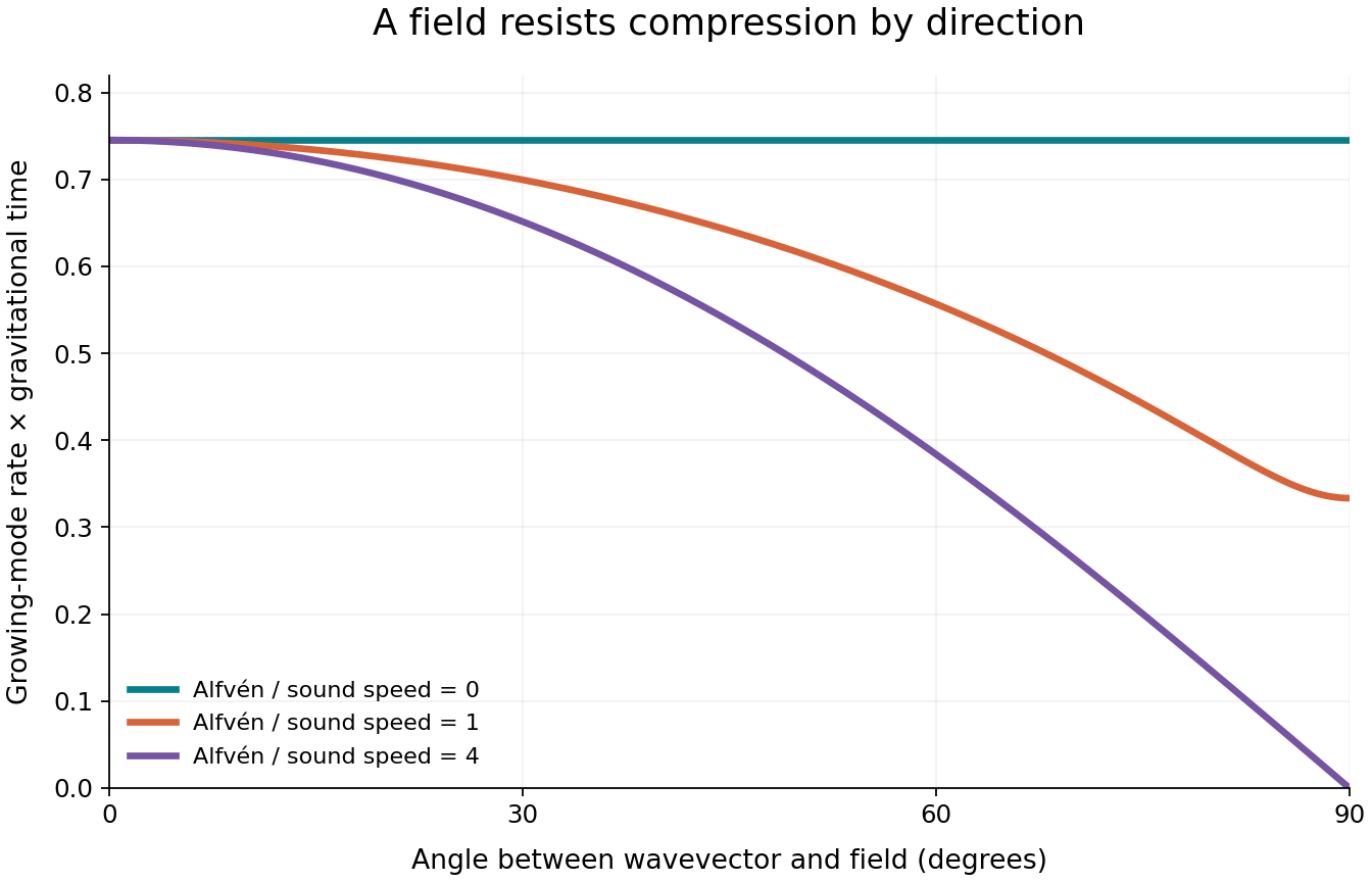
For $\theta=0$, the compressive branch recovers $\omega^2=c_s^2k^2-\omega_J^2$ from L1. Increasing the field leaves that parallel Jeans threshold unchanged. At exactly $90^\circ$, the nonzero compressive frequency contains $c_s^2+v_A^2$ because magnetic pressure participates in the restoring force.

Take field strength to zero as another check. The quartic separates a $\omega^2=0$ branch from the ordinary Jeans branch, and the Alfvén frequency vanishes. Transverse velocity may stay constant; density compression returns to L1. This limit can reveal an extra field-strength factor in an implementation.

Reading: Chandrasekhar & Fermi 1953, Problems of Gravitational Stability in the Presence of a Magnetic Field · Molecular-cloud Jeans standalone scientific reproduction

Calculate a strong-field example

Use $J=1.5$, a box-spanning fundamental wave, and $v_A/c_s=4$. Solve the quadratic in frequency squared. The parallel growth rate is $0.745356/t_0$. At $45^\circ$ it falls to $0.537226/t_0$, and at $89^\circ$ it is $0.0135481/t_0$. These values are recomputed from the quartic in the worked-example program.

The last rate is small and positive. A finite-duration record near the perpendicular direction can therefore show very little slow growth. The exact $90^\circ$ endpoint includes neutral and oscillatory branches. A tiny positive real part left by floating-point arithmetic needs a scale-aware neutral classification.

The saved field example starts from a longitudinal displacement with $b_y=B_y\delta$, zero velocity and density amplitude $0.02$. This generally excites a combination of modes. Each listed rate belongs to a mode; the integrated six-component state determines how their contributions combine in the density history.

Reading: Molecular-cloud Jeans standalone scientific reproduction

Check every disturbance before extending a linear calculation

A small density contrast alone does not guarantee that the entire disturbance remains small. Density may briefly pass through zero contrast even though velocity or magnetic disturbance has grown. The examples track density, relative field disturbance and normalized velocity, stopping before a specified small-amplitude cap is crossed.

Velocity is normalized by $\sqrt{c_s^2+v_A^2}$, and the relative cap is $0.15$. This speed defines a stopping scale. Propagation and growth still come from the six equations with their directional magnetic force.

The nonmagnetic gas patch evolves finite-amplitude mass and momentum. This calculation evolves linear magnetic disturbances on a uniform background. Their distinct assumptions let you choose the calculation that answers the particular question you are asking.

Reading: Molecular-cloud Jeans standalone scientific reproduction

A directional wave test differs from a cloud’s magnetic criticality

A question about supporting an entire cloud also needs a shape, a surface through which to measure magnetic flux, and a specification of the external field. Published critical mass-to-flux ratios carry those geometric assumptions. One periodic wave does not define a universal critical cloud mass.

In this uniform model, allowing a wavevector along the field leaves the original Jeans-unstable compressive direction available. The paper guide later examines three-dimensional turbulent simulations, where flows in many directions accompany a separate question about characteristic masses and resolution.

Reading: Guszejnov et al. 2020, Can magnetized turbulence set the mass scale of stars? arXiv:2002.01421v1 · Federrath & Klessen 2012, arXiv:1209.2856v1