Find the model before reading the curve
Open Giomi’s version 2, dated 3 August 2015. Equation (1) specifies a coupled nematic–fluid model; Section I.2 introduces the active length from elastic and active stresses. Its square-root scaling estimates where those stresses balance. It is a scale relation, not a universal coefficient for a biological sample.
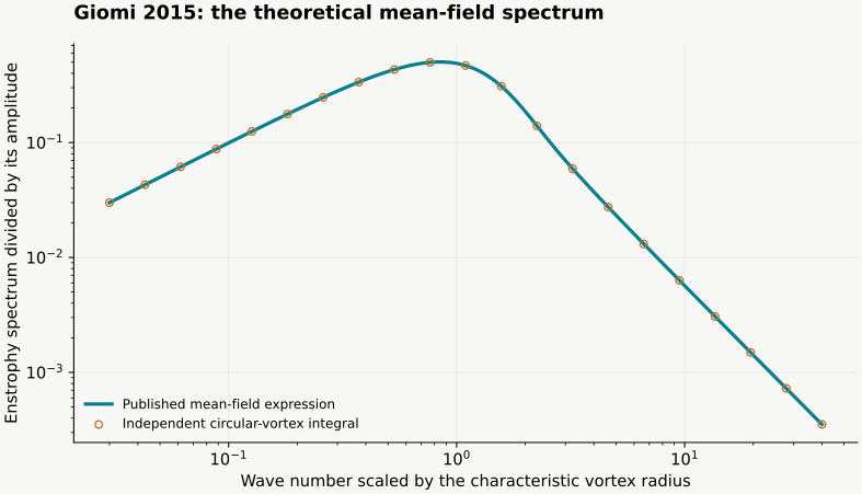
Figure 5C–D shows numerical enstrophy and energy spectra at three activities. The following mean-field calculation describes their scaling. The mean-field construction treats vortices as uncorrelated circular objects with an exponentially distributed area. Our reproduction evaluates the normalised theoretical enstrophy curve in equations (9) and (14). The reproduction contains the calculated curve and its independent integral check.
Recalculate the spectrum by two routes
Enstrophy measures squared vorticity. Its spectrum distributes that quantity over wave number. Scale wave number by the characteristic vortex radius and divide out the normalisation constant. The resulting dimensionless curve can be computed from modified Bessel functions, or from an independent integral over vortex radii.
The plot below is calculated from that theoretical expression. The independent quadrature checks the special-function evaluation. Small wave numbers have a slope approaching positive one on logarithmic axes; large wave numbers approach minus two. The horizontal scale is dimensionless. Neither axis is an experimentally calibrated time or length.
Worked example
Use a simple flow to understand the tracer diagnostic
A flow map assigns each starting point its position after a chosen time interval. Its derivative describes how an initially small patch deforms. Multiply that derivative by its transpose in the correct order to form the right Cauchy–Green tensor. Its largest eigenvalue gives the square of the strongest local stretching factor.
For a planar area-preserving extension, one coordinate grows exponentially and the other shrinks at the same rate. The largest finite-time Lyapunov exponent equals the extension rate. This worked example has no defects and no active stress: it checks the kinematic diagnostic independently of the physics that generated the velocity.
Read the 2023 figures in material coordinates
Open Serra and colleagues, DOI 10.1038/s41567-023-02062-y, published 25 May 2023. Figure 1 distinguishes initial positions from final positions and sketches stretching and folding. Equations (1)–(3) define the flow map and finite-time stretching. Figure 2 applies the analysis to measured microtubule–kinesin velocities, using a 100-second interval for the illustrated forward and backward maps.
A forward map starts at initial positions and quantifies separation; a backward map starts at final positions and diagnoses convergence over the same interval. Compare labels before comparing ridges. The linked browser model supplies synthetic Q fields, velocities and tracers for a separate numerical experiment.
Choose the next reproducible comparison
To test the theoretical spectrum, keep its vortex assumptions and compare the two numerical evaluations. To test a continuum solver, use the manufactured sinusoidal force-to-flow example and refine the grid. To investigate defect control, compare matched trajectories and the chosen flux with and without anchoring. These checks answer different questions and belong beside the result they support.
For the next paper, write down the version, the figure and axis units, what was measured or simulated, and which parameters are specified. Choose a comparison you can calculate independently. Save the seed, initial field, numerical resolution and observation interval before interpreting a new pattern.