Reanalyze twenty-five measured Kepler-289 transit times

Read the two kinds of time in Table 1

The file ajac8553t1_mrt.txt has a planet name, a number, an observed mid-time and error, then a predicted mid-time and a different error. Blank observed fields mean there is no measurement in that row. The prediction error belongs to a dynamical forecast, not an independent telescope measurement.

The original revision 1 file is 25,058 bytes. Its SHA-256 is preserved in the downloadable provenance and checked before selection. It contains 466 rows, of which 51 have both an observed time and a positive observed error. The other 415 are prediction-only rows. The extraction keeps all 51 measurements for inspection.

There are two source defects to handle explicitly. The number column is a global row counter, despite being described as a transit epoch; subtract 0 for b, 259 for d and 395 for c to obtain per-planet epochs. The paper describes a 2021 WIRC transit, but source row 430 has a blank observed column. Its forecast must remain excluded. The 2019 WIRC time is present at 4719.7411 days with 0.0026-day uncertainty.

Reading: Greklek-McKeon et al. · Greklek-McKeon et al.

Freeze one measured sample for both fits

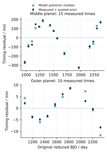
Select current Kepler-289d and Kepler-289c, retain only rows with observed time and uncertainty, and require reduced BJD below 3000. That gives 15 middle-planet and 10 outer-planet Kepler measurements. Both competing likelihoods use these same 25 values and their original errors. No measurement is removed because a model fits it poorly.

Names have changed since the 2014 PH3 discovery paper: its PH3c is today's middle Kepler-289d, while PH3d is today's outer Kepler-289c. Period and position in the system are safer labels than a bare letter when comparing the older chopping demonstration with the newer table.

Keep the source time coordinate as BJD minus 2454000 days. The MRT labels it JD and neither obtained text states UTC versus TDB. The scripts do not invent that conversion. The four-decimal-day time resolution is 8.64 seconds, distinct from the supplied timing errors. The missing shared timing covariance makes the diagonal likelihood an explicit approximation.

            python3 verify-observations.py --input .

Reading: Greklek-McKeon et al. · Schmitt et al. · Greklek-McKeon et al.

Keep the clock inside the inference

For a display plot, fit a weighted linear ephemeris and show early/late residuals with the quoted timing error bars. The mass likelihood itself uses the original times. Treating residuals from an estimated clock as independent new measurements would lose the correlation introduced by fitting that clock.

The fitted parameter set has nine dimensions: two masses, two components of the free-eccentricity combination, a period and central linear-ephemeris epoch for each planet, and one common positive white-jitter scale. The central epochs are nominal clock times at integer epochs 10 and 5; actual crossings also include the perturbation. This centering reduces epoch–period correlation during sampling.

The adopted stellar mass is fixed at 1.08 solar masses for the conversion to Earth masses. Its published uncertainty is not propagated here. The direct dynamical information is a planet-to-star mass ratio; absolute masses remain conditional on this stellar scale.

\vartheta=(m_d,m_c,\operatorname{Re}Z_{\rm free},\operatorname{Im}Z_{\rm free},T_{d,10},T_{c,5},P_d,P_c,s)

The periods, epochs, uncertainties and jitter all use days. The two mass coordinates use Earth masses. No photometric forecast from Table 1 is a prior on these parameters.

Reading: Lithwick · Greklek-McKeon et al.

Declare the harmonic model and its prior

The baseline calculation uses the zero-free-eccentricity chopping formula through eight harmonics, plus only the free-eccentricity slow correction. The slow-only comparison retains the aliased inner second and outer first harmonics. This removes the independent chopping information without adding the forced resonant contribution twice.

Mass priors are uniform over 0.05–60 Earth masses for the middle planet and 5–600 for the outer. Each free-vector component has a zero-mean Gaussian prior of width 0.03, truncated at 0.15 in either direction. Period and central-epoch priors are finite uniforms with the exact bounds in timing-results.json. Jitter has a half-normal prior of thirty minutes, restricted to the stated positive interval.

The likelihood includes the variance normalization. The sampler uses differential-evolution proposals, conditional Gaussian updates for the linear eccentricity terms and a slice update for log jitter. Truncated eccentricity draws are rejected outside their support; finite positive mass conditionals use the truncated normal distribution. Log-mass and log-jitter proposals include their change-of-coordinate Jacobians.

These support bounds define a mathematical approximate model. They do not certify every allowed eccentricity combination against a full three-planet orbit. Larger free-vector values and the broad-prior run are especially important to inspect against the low-eccentricity approximation.

Reading: Deck & Agol · Lithwick · Greklek-McKeon et al.

Download the public files and reproduce

The download script reads a public allowlist, checks every byte count and SHA-256, and creates a self-contained directory. It retrieves the original table, scripts, saved outputs and compressed chains. The website's private repository and interactive Engine are unnecessary.

Run the short observation and frozen-chain checks first. The orbit script separately recreates the synthetic default with a standard-library Newtonian integrator; this is a numerical teaching experiment, not an analysis of the measured Kepler times. The final command reruns the actual timing posterior with four independent thirty-walker ensembles.

To repeat the full comparison and both sensitivity experiments, run run-frozen-inference.py. One run uses the same observed data with a wider free-eccentricity prior; another is a labeled analytic-model injection at the same integer epochs and errors. Injection outputs keep the original observed times in their own column and label the replaced analysis times as synthetic.

            curl -fsS -O https://sandboxphysics.com/stories/transit-timing/download-tutorial.py
python3 download-tutorial.py --directory ac19
cd ac19
python3 verify-observations.py --input .
python3 reproduce-orbits.py --out new-orbit
python3 analyze-frozen-posterior.py --directory .
python3 reproduce-timing.py --input . --out new-posterior --iterations 16000 --ensembles 4

Reading: Greklek-McKeon et al. · Deck et al. · Deck & Agol

Read the interval alongside the discrepancy

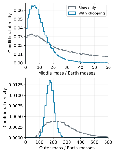
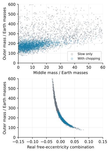
The table below is generated from the saved posterior summaries. Brackets mark the sixteenth and eighty-fourth percentiles, not hard bounds and not a coverage statement for the true system. Adding chopping narrows the outer planet's conditional distribution and changes the middle planet's broad mass ridge.

Now read the residuals and jitter. The approximate model needs extra scatter of order fifteen minutes even with chopping; the supplied outer-planet measurement errors are typically well below a minute. The raw-error residual sum of squares remains several hundred at a representative posterior draw. That statistic is not a minimized chi-square and is not assigned a frequentist probability.

The physical result is a substantial inadequacy of this reduced two-planet harmonic description at the quoted measurement precision. A narrower conditional interval describes the chosen model and scatter prescription. It cannot replace the published three-planet analysis or justify its level of physical mass accuracy.

Approximate model	Middle mass, Earth units	Outer mass, Earth units	Median extra scatter / min
Slow harmonics only	$17.5\;[5.07,41.2]$	$246\;[155,367]$	27.9
With chopping	$8.56\;[3.24,17.0]$	$178\;[149,208]$	15.6

Reading: Deck & Agol · Greklek-McKeon et al. · Greklek-McKeon et al.

Look for failure before looking for precision

Inspect independent ensemble traces and the saved diagnostic for their iteration-mean agreement. Values close to one are useful evidence of agreement, not proof that every mode was explored. Effective ensemble means count averaged, correlated ensemble iterations; they are not the number of independent walker samples.

The first wide-prior sampler exposed a second poorly mixed mode. Conditional updates and log-jitter slice sampling were added, and the frozen runs retain the final diagnostics. The earlier failure is described in the verification report. The same-data wider-prior calculation tests whether a mass ridge has been hidden by the narrower eccentricity assumption.

The analytic injection uses known masses of six and 150 Earth masses and a declared free vector, then adds noise with the original timing errors. It tests closure of the approximate inference at the same sparse sampling. It is not an independent validation of the harmonic physics; that check uses actual Newtonian events and a separate IAS 15 calculation. A single injection also does not measure interval coverage.

For the next dataset, record the time standard, measured/predicted columns, integer gaps, likelihood normalization, prior support, chain agreement and model residuals. Those seven items let a mass interval be read as a physical claim with a defined scope.

Reading: Deck et al. · Deck & Agol · Greklek-McKeon et al.

Take the calculation with you

Twenty-five measured transit residuals with quoted errors and reduced-model posterior medians — The points are measured times relative to each planet’s fitted linear clock. Crosses summarize the reduced harmonic model. The large remaining mismatch matters even when a conditional posterior is narrow.

Conditional mass densities under the slow-only and chopping models — Both calculations use the same fifteen middle-planet and ten outer-planet measurements. Chopping changes the conditional mass information within a two-planet approximation whose remaining discrepancy is visible above.

Retained correlated posterior draws showing mass and free-eccentricity dependence — These are correlated draws, with four independent ensemble runs per model. Inspect the saved diagnostics and wider-prior experiment before interpreting an interval.

Download the small fetcher below and run it in an empty directory. It retrieves only the scientific allowlist, checking every file’s byte count and SHA-256 hash. Python 3.9 or later suffices for the main calculation; no account or repository checkout is needed.

download-tutorial.py · Exact file manifest · Commands and numerical comparison

# Save download-tutorial.py from the link below, then:
python3 download-tutorial.py --directory kepler289-timing
cd kepler289-timing
python3 verify-observations.py --input .
python3 verify-inference.py --input .
python3 analyze-frozen-posterior.py --directory .
python3 reproduce-orbits.py --out new-orbit
# The full six-run posterior calculation takes substantially longer:
python3 run-frozen-inference.py --input . --out new-all

The compressed chains retain all 63,960 correlated draws per model. Regenerating the posterior is a Monte Carlo calculation. Draw sequences can differ across math libraries; numerical summaries and diagnostics provide the reproducibility checks. The frozen analytic injection is a separate inference-closure exercise.

All public inputs, scientific scripts and frozen outputs

download-tutorial.py (2 KiB)
reproduce-timing.py (7 KiB)
run-frozen-inference.py (1 KiB)
timing_data.py (3 KiB)
chopping_model.py (5 KiB)
timing_posterior.py (4 KiB)
timing_priors.py (2 KiB)
timing_conditionals.py (5 KiB)
posterior_diagnostics.py (3 KiB)
analyze-frozen-posterior.py (4 KiB)
nbody_timing.py (5 KiB)
reproduce-orbits.py (2 KiB)
verify-observations.py (2 KiB)
verify-inference.py (3 KiB)
verify-ias15.py (4 KiB)
validate-harmonics.py (3 KiB)
plot-timing.py (6 KiB)
posterior-slow-samples.csv.gz (3055 KiB)
posterior-chopping-samples.csv.gz (3010 KiB)
posterior-timing-results.json (14 KiB)
posterior-selected-times.csv (2 KiB)
prior-sensitivity-slow-samples.csv.gz (3054 KiB)
prior-sensitivity-chopping-samples.csv.gz (3011 KiB)
prior-sensitivity-timing-results.json (14 KiB)
prior-sensitivity-selected-times.csv (2 KiB)
injection-slow-samples.csv.gz (3004 KiB)
injection-chopping-samples.csv.gz (2889 KiB)
injection-timing-results.json (14 KiB)
injection-selected-times.csv (3 KiB)
analysis-summary.json (17 KiB)
default-model-check.json (47 KiB)
harmonic-validation.json (1 KiB)
observation-offsets.json (3 KiB)
reference-input.json (144 KiB)
provenance.json (5 KiB)
numerical-reference.json (219 KiB)
synthetic-orbit.json (16 KiB)
ajac8553t1_mrt.txt (25 KiB)
kepler289-observed.csv (2 KiB)
source-attribution.txt (3 KiB)
reproduction-readme.txt (3 KiB)
kepler289-measured-timing.svg (61 KiB)
kepler289-conditional-masses.svg (60 KiB)
kepler289-mass-degeneracy.svg (1112 KiB)

The author’s machine-readable table is attributed under CC BY 4.0; original scientific scripts use MIT. The attribution file records versions, source links and the distinction between measured times, synthetic orbits and model-dependent inference.

Try the observation

Compare a controlled orbit with the measured inverse problem

Export the default synthetic orbit and compare its perfect-model timing pattern with the real sample's residual scatter.
Use the eccentric preset to see why changing a physical orbit can alter the slow timing wave before any noise is added.
Keep the synthetic trajectory, actual measured times and analytic injection in separate files when rerunning the tutorial.

Sources and calculation scope

Lithwick, Xie & Wu, Extracting Planet Mass and Eccentricity From TTV Data (2012)
Pinned v2, Sections 2.1–2.3, Equations 1–10 and Appendix B. The free-eccentricity vector and the near-resonant validity conditions.
Deck & Agol, Measurement of Planet Masses with Synodic Chopping (2015)
Pinned v1, Sections 2–5.1, Equations 10–15 and Appendix A. The transit sampling aliases some harmonics; the PH3 application explicitly compares mass constraints with and without chopping.
Deck et al., TTVFast (2014)
Pinned v1, Sections 2.1.3, 2.2–2.3 and 3. Mid-transit is a foreground minimum of astrocentric sky separation. This teaching calculation reuses the site's RK4 kernel and independently checks IAS15; it does not port the GPL TTVFast code.
Greklek-McKeon et al., Kepler-289 Densities and Transit Timing (2023)
Pinned v1, Sections 2–3, Table 1 and Figures 2–4, 9–10. CC BY 4.0. The author analysis jointly fits transit shapes, then fits the measured times with a three-planet dynamical model.
Greklek-McKeon et al., original Table 1 machine-readable file
Revision1, 25,058 bytes; SHA256 8f958e773fae5a6d17aa090c5d523e13829f6b69a2f3d51ceecbf5e2d0d56af9. Fifty-one measured rows are distinct from 415 prediction-only rows. The 2021 WIRC observation is absent from the observed column.
Schmitt et al., Planet Hunters VII and PH3 (2014)
Pinned v1, the transit/dynamical analysis and Table 5. PH3c is today's Kepler-289d, while PH3d is Kepler-289c. The older forecast table is not used as an independent measurement list.